该文在清醒猕猴下颞皮层(IT)单细胞记录中检验了神经元对真实材质图像的编码机制。研究涵盖三个递进维度:首先检验 IT 神经元对真实材质纹理是否具有独立于轮廓形状的选择性;其次通过改变光照方向测定材质选择性的光照不变性;最后利用随机相位对照图像排除了单纯傅里叶功率谱与平均亮度对纹理选择性的解释。
研究背景
物体识别研究长期以形状为主要入口,但日常视觉还必须判断东西由什么材料构成。相同轮廓可以由木材、金属或织物形成,材料信息也会改变我们对可食性、表面状态和操作方式的判断。此前的下颞叶研究已证明复杂形状和颜色能够调制神经元反应,人工纹理实验也显示表面模式并非被高级视觉皮层忽略。然而,真实材料的识别不能完全归结为颜色:即便只保留灰度,明暗纹理和高光仍可传递材质线索。因而,要理解下颞叶支持的视觉表征,需要把轮廓之外的表面图像结构纳入测量。
真实材料同时带来一个人工纹理不易暴露的难题。其微观起伏和反射特性会使图像随照明方向显著改变,同一块材料在不同光照下的亮度分布,可能比不同材料之间还不相似。对一张材料照片反应强,只能证明图像选择性,不能证明稳定的材料表征;若偏好在光照改变后仍保持,才更接近知觉中的材料恒常性。另一个问题是形状与材质如何共同编码:二者可以由不同细胞群承担,也可以在同一神经元上表现为相对可分离的调谐。仅分别测试两类刺激,无法区分这些组织方式。功率谱、平均亮度及对比度还可能造成表面上的材料差异,需要通过保留部分图像统计而破坏其空间结构的对照来限定解释。
本文使用真实材料数据库中的灰度图像,将多种材料与不同轮廓交叉组合,再改变材料的照明方向,分别测量纹理与形状的可分离性以及跨光照的稳定程度。随机相位图像用于检验功率谱之外的结构是否参与神经选择性,人类相似性分类和猴神经群体解码则提供不同层面的参照。这样的设计允许观察到单细胞不变性有限而群体仍有可读出信息,两者并不矛盾。但实验猴仅执行注视,未在这些条件下报告材料知觉;每种材料每个照明方向的图像取样也有限,不能把对有限照片的分类直接扩大为对整个材料类别的抽象认识。本文所推进的是下颞叶对真实表面信息的编码及其变换容忍度,而非已经证明了完整的材料恒常性机制。
研究思路
作者的设计是两条正交的刺激轴加上一个低层控制。第一,形状 × 纹理:12 种真实材料的图像(毛圈布、砂纸、石膏、铝箔、生菜叶、瓦片、盐晶、亚麻、混凝土、白面包等)与 5 种轮廓形状全交叉成 60 个条件,从单细胞反应的方差分解出形状主效应、纹理主效应与交互,并用可分离性指数 S 判断两套调谐是否互不干扰。第二,光照方向:每种材料从三个仰角(22.5°、45°、67.5°,方位角 0°)成像,考察材料选择性对光照的不变性。第三,随机相位控制:对每张图像做傅里叶变换,保留功率谱、随机化相位谱后反变换,若神经元对原图与对照的反应不同,则说明选择性不依赖功率谱(含平均亮度)——因为对照组的功率谱与原图几乎相同。作为"外部参照",作者还让 36 名人类被试对 36 张图做自由相似性分类,用于对比"知觉层面的光照不变性"与"神经层面的光照不变性"。最后用支持向量机(Support Vector Machine, SVM)做群体解码,定量回答"这些神经元的群体反应能否跨光照方向分类材料"。
方法
两只幼年恒河猴,在前部 IT(区域 TE:前部上颞沟下岸与外侧凸面)做标准胞外单细胞记录;动物只需完成注视任务(不要求辨别或分类刺激):注视小点 0.12°,刺激呈现 200 ms,试次间隔约 1000 ms,保持注视才有间断的苹果汁奖励,仅分析注视保持完好的试次。刺激取自 CURET 真实材料图像库(正对视角),转为灰度并做 gamma 校正;每张材料图与 5 种形状(约 4.5°)交叉。正式测试有两个:shape_texture 测试在同一天内固定一个光照方向,交错呈现 12 纹理 × 5 形状共 60 个条件(每条件约 10 次);illumination_direction 测试选取该神经元在线看出的最佳形状,交错呈现 36 张原图(12 材料 × 3 方向)加 36 张随机相位对照图。数据分析以刺激后 50–250 ms 为响应窗、刺激前为基线窗;用双因素方差分析检验形状/纹理(或材料/光照方向)主效应与交互,以关联强度指数 χ² 度量选择性大小(兼顾均值与试次间变异),以可分离性指数 S(乘法模型预测调谐的方差解释率,置换检验定显著)判断两维调谐是否独立;SVM 解码沿用 Hung 等(2005)的思路,以 106 个神经元 50 ms bin 的拼接反应向量为输入、C-SVM 加径向基核,70% 试次训练、30% 测试,训练与测试可在相同或不同光照方向间进行,重复 100 次取平均,偶然水平 1/12≈8.3%。
主要结果
- 材料纹理是 IT 神经元的实质性编码维度。125 个响应神经元中,77% 有显著形状主效应,84% 有显著纹理主效应;但选择性强度上纹理(中位 χ²=0.08)大于形状(中位 χ²=0.04),交互很小(中位 χ²=0.02),且两维选择性之间呈显著负相关(r=−0.30,P<0.001)——形状选择强的细胞纹理选择弱、反之亦然(图 3、图 4)。多数反应无法用平均亮度解释(如某神经元偏好较暗的 d、e、l 纹理却对亮度相仿的 g 无反应)。
- 两维调谐可分离。对同时调谐于形状与纹理的神经元,S 指数中位数达 0.81(ANOVA 标准入选的 89 个,全部显著高于随机置换水平;表 2);图 5 显示这 12 个双调谐细胞的纹理偏好在各形状间几乎不变,形状偏好在各纹理间同样如此——即"最佳纹理不因形状而变,最佳形状不因纹理而变",类似 V1 神经元朝向调谐不随空间频率改变。剔除生菜叶后结论不变(S=0.71)。
- 光照方向强烈影响反应,不变性普遍偏弱。光照方向测试的 127 个响应神经元中,83% 有材料主效应,48% 有光照方向主效应,65% 有二者交互(图 6–8);同种材料换一档光照(差 22.5°)反应平均变化 1.5 倍、换两档(差 45°)变化 1.7 倍(响应性指数中位数 0.19 与 0.25)。材料 × 光照的调谐可分离性中位数仅 0.59,只有约一半细胞达显著(表 3);光照偏好甚至会在材料排名两端反转(图 9A)。12 种材料中砂纸的光照不变性最高(群体神经距离均值 0.27,表 4)。
- 群体层面能跨光照方向解码材料,但远不如同光照条件。SVM 用一个方向训练、另一方向测试时,相邻方向间正确率约 40–50%,相差最大的两方向(22.5° vs 67.5°)降至约 23–31%,而偶然水平仅 8.3%;同方向训练测试则达 65–97%(表 5、图 10)。大部分解码信息在刺激后 200 ms 内已经可用(延长窗口仅提升约 5%)。生菜叶在全部六组训练—测试组合中几乎被完美分类,砂纸与混凝土次之(图 11)。剔除生菜叶后跨方向性能降至 17–54%,仍高于偶然。
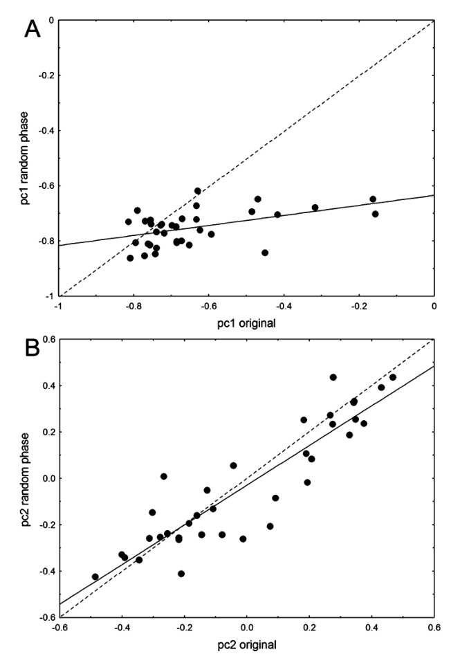
- 纹理选择性需要相位信息。112 个纹理选择神经元中 82% 对相位随机化有显著主效应或交互(中位 P 低至 0.00003);PCA 显示 PC1(解释 45% 方差)上原图与随机相位图显著分离(坐标相关仅 r=0.48,Wilcoxon P<0.000025),而 PC2(9% 方差)上两者几乎重合(r=0.90)且与平均亮度(r=0.68)和均方根对比度(r=−0.67)相关(图 12–14)。由于原图与对照的功率谱差异小于任意两张原图间的差异,PC1 的分离不能归因于功率谱的微小残余差别——亮度/功率谱因素合计解释不到 10% 的方差,材料纹理选择性主要依赖相位结构所载的高阶图像特征。
图注解读
图 1 · 刺激材料总览
原文图注:Fig. 1. Stimuli. (A) Images of the 12 materials illuminated from an elevation of 45°: (a) terrycloth, (b) sandpaper, (c) plaster, (d) aluminium foil, (e) lettuce leaf, (f) plaster (zoomed), (g) roof shingle, (h) salt crystals, (i) linen, (j) concrete, (k) white bread and (l) soleirolia plant. (B) Images of one material (terrycloth) combined with each of the five shapes employed.
A 面板给出 45° 仰角下的 12 种材料样例(a–l 为后文所有分析的字母标签),B 面板展示同一材料(毛圈布)嵌入 5 种轮廓形状的效果。它定义了全文的刺激命名体系,支撑方法与结果中"12 纹理 × 5 形状"的设计描述。
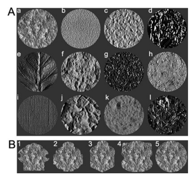
图 2 · 光照方向与相位随机化的操纵
原文图注:Fig. 2. Stimuli: manipulation of illumination direction and phase randomization. (A) Two materials shown for each of the three illumination directions (columns). Illumination direction condition 1, 2 and 3 refers to an elevation of 22.5°, 45.0° and 67.5°, respectively (azimuth: 0°). (B) Original and random phase version of the lettuce leaf image. (C) Original and random phase version of the sandpaper image. Note the more salient effect of the phase randomization for the lettuce leaf (B) compared with the sandpaper image (C).
A 面板并排呈现两个材料在三个仰角下的外观差异,B、C 面板对比生菜叶与砂纸的原图及其随机相位版本——生菜叶的相位随机化效果远比砂纸醒目。这张图直观说明两点:光照方向确实改变了材料图像的外观;相位控制操作的视觉后果依材料而异,为结果第 5 条的相位分析提供了感性基础。
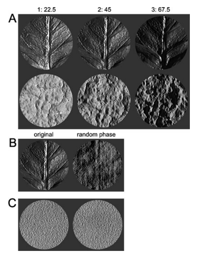
图 3 · 单细胞示例:纹理调谐与形状调谐的三种类型
原文图注:Fig. 3. Selectivity of IT neurons to 'material textures' and shape: single neuron examples. Peristimulus time histograms of the responses of single IT neurons to the 60 combinations of five shapes and 12 textures (shape_texture test). The stimuli in a row or column depict the same shape or texture, respectively. The numbers (shapes; rows) and letters (textures; columns) refer to the shapes and textures of Fig. 1A, respectively. Vertical lines in each histogram indicate stimulus on- and offset. (A) Neuron tuned to material texture but less so to shape. (B) Neuron tuned to shape but less so to material texture. (C) Neuron tuned to both texture and shape properties.
三个神经元的围刺激时间直方图(peristimulus time histogram, PSTH)阵列:行是形状、列是纹理。读法是看"按行扫描变化大"还是"按列扫描变化大"——A 细胞列间差异悬殊(纹理主导),B 细胞行间差异悬殊(形状主导),C 细胞两者都强。这张图给结果第 1 条提供了最直接的细胞个案。
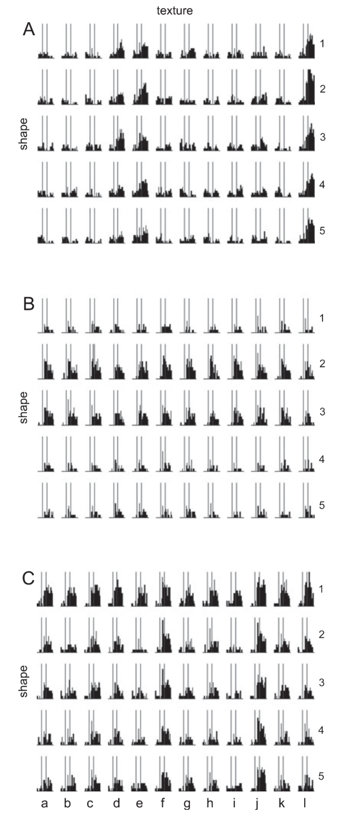
图 4 · 纹理与形状选择性的对比
原文图注:Fig. 4. The degree of texture and shape selectivity compared for the responsive neurons in the shape_texture test (n = 125). (A) The anova-based χ2 for texture plotted against that for shape. B. The texture selectivity indices (computed following Komatsu & Ideura, 1993) plotted against the shape selectivity indices. The values of the two animals (M1 and M2) are plotted using different symbols.
A 面板横轴为形状 χ²、纵轴为纹理 χ²,散点明显沿坐标轴聚集成"L"形而非对角线:多数细胞只在其中一个维度上选择性大,且两指数负相关(r=−0.30)。B 面板改用 Komatsu & Ideura 的 best/worst 选择性指数,两者仅弱正相关(r=0.23)。两张散点图合起来支撑结果第 1 条的"独立编码"结论。
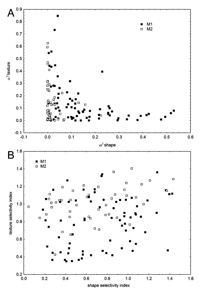
图 5 · 双调谐细胞调谐可分离性的可视化
原文图注:Fig. 5. Mean responses as a function of texture and shape rank for the neurons (n = 12) that show a selectivity index, χ2, larger than 0.10 for both shape and texture, or an interaction χ2 larger than 0.10. The shape rank is indicated by different symbols, with rank 1 corresponding to the shape with the largest mean response. Error bars indicate 95% confidence intervals.
对 12 个双调谐细胞按净反应做排名平均:横轴为纹理排名,不同符号为形状排名,纵轴为平均反应。若两维调谐纠缠,形状曲线会随纹理排名散开;实际图中不同形状的曲线几乎平行——纹理偏好在形状间保持,形状偏好在纹理间保持。这张图是结果第 2 条"可分离性 S=0.81"的图形化呈现。
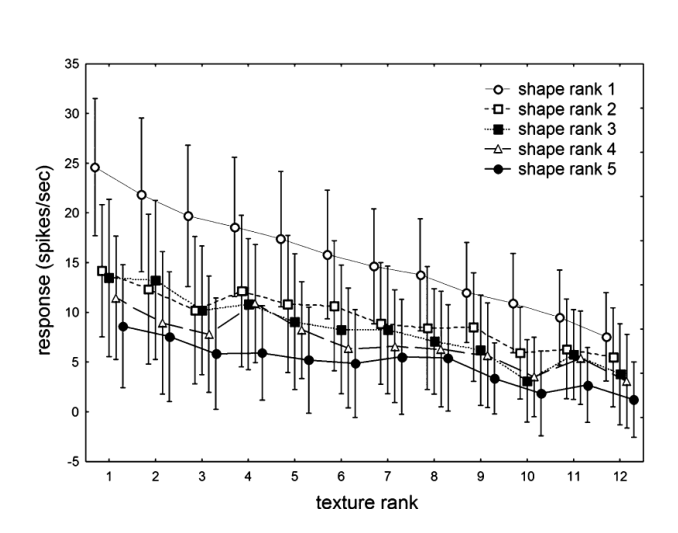
图 6 · 光照方向对单个 IT 神经元的影响
原文图注:Fig. 6. Effect of illumination direction on the responses of a single IT neuron to images of materials. Peristimulus time histograms of the responses of a single IT neuron to the 36 combinations of 12 materials and three illumination directions. The stimuli of a row and column depict the same illumination direction and material, respectively. The letters (materials; columns) refer to the materials of Fig. 1A, while the numbers indicate the illumination directions in degrees of elevation. Vertical lines in each histogram indicate stimulus on- and offset. This example neuron showed a strong effect of material and illumination direction.
示例神经元在 67.5° 仰角下对材料反应强烈而选择,22.5° 下几乎无反应,45° 下只对部分材料反应。行间(光照)差异一目了然,说明光照方向本身就能开关一个细胞对整组材料的反应。它支撑结果第 3 条中"光照方向强烈影响反应"的论断。
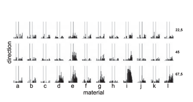
图 7 · 光照与相位的联合影响:示例 1
原文图注:Fig. 7. Effect of illumination direction and phase randomization on the responses of a single IT neuron: single neuron example 1. Peristimulus time histograms of the responses of a single IT neuron to the 36 combinations of 12 materials and three illumination directions for the original (top) and random phase images (bottom). The stimuli of a row and column depict the same illumination direction and material, respectively. The letters (materials; columns) refer to the materials of Fig. 1A, while the numbers indicate the illumination directions in degrees. Vertical lines in each histogram indicate stimulus on- and offset. This example neuron showed effects of material, illumination direction and phase randomization.
上排为原图、下排为随机相位对照:同一材料、同一光照方向下,上下两排的反应可以差别悬殊。由于两张图的功率谱几乎相同,这种差别只能来自相位信息。它为结果第 5 条提供细胞个案。
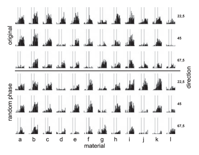
图 8 · 光照与相位的联合影响:示例 2
原文图注:Fig. 8. Effect of illumination direction and phase randomization on the responses of a single IT neuron: single neuron example 2. Same conventions as in Fig. 7. This example neuron responded selectively to the lettuce leaf for the three illumination directions and showed a strong effect of phase randomization.
这个细胞对生菜叶在三个光照方向下都选择性强反应——是全文少见的接近"光照不变"的个案;但同条件下它对混凝土(j)的反应只在 67.5° 出现,说明不变性并不彻底。相位随机化也强烈改变其反应。支撑结果第 3、5 条。
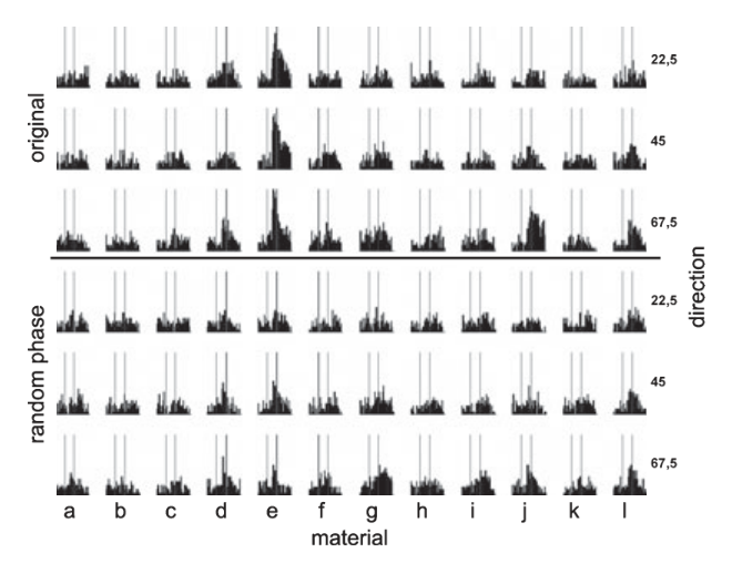
图 9 · 群体平均反应:材料与光照方向
原文图注:Fig. 9. Mean responses as a function of material and illumination direction. (A) Mean responses as a function of material and illumination direction for the 68 neurons that demonstrated a χ2 of at least 0.10 for the main effect of materials or the interaction of the two factors. The illumination direction rank is indicated by different symbols, with rank 1 corresponding to the illumination direction with the largest mean response. (B) Mean net response strength for all neurons (n = 127) responsive to at least one of the 12 materials for each of the three directions of illuminations. The materials are labelled as in Fig. 1 and the illumination directions are indicated as given in the legend. Error bars indicate 95% confidence intervals.
A 面板把每个细胞的材料偏好与光照偏好分别排名后平均:光照偏好曲线在不同材料间大体平行,但在材料排名的两端(最佳与最差材料)发生反转,提示调谐可分离但分离不完全。B 面板为 127 个细胞对每种材料三个方向的净反应均值:生菜叶与混凝土群体反应偏大,但 Bonferroni 校正后材料间两两差异均不显著。支撑结果第 3 条。
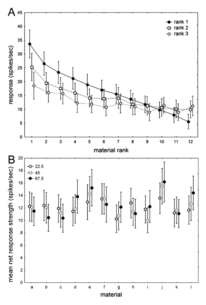
图 10 · SVM 跨光照方向分类材料的性能
原文图注:Fig. 10. Classification performance of materials across illumination direction with Support Vector Machines that use IT responses as input. Per cent correct classification is plotted as a function of the end of the analysis window. The start of the analysis windows was always 50 ms. Full lines: SVM trained and tested with the same illumination direction. Stippled lines: SVM tested with an illumination direction other than the trained one. For A, B and C the trained illumination directions were 1, 2 and 3, respectively. In the case of the stippled lines, the tested illumination directions were 2, 3 and 1, respectively. Chance performance is indicated by the horizontal dashed-dotted line. Error bars indicate standard deviations on the average per cent correct classifications across 100 permutat…
横轴为分析窗终点(50 ms 起,200–400 ms),纵轴为分类正确率;实线是同方向训练+测试,虚线是跨方向测试,虚线由高到低依次为相邻方向与最远方向,水平虚点线为偶然水平 8.3%。关键读法:虚线远高于偶然水平但显著低于实线,且距离越远越低;窗口延长只带来约 5% 提升。支撑结果第 4 条。
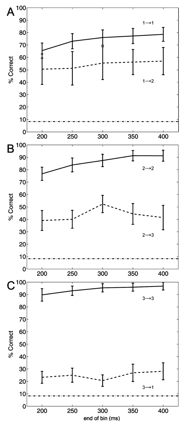
图 11 · SVM 分类的混淆矩阵
原文图注:Fig. 11. Classification performance of materials across illumination direction with Support Vector Machines that use IT responses as input: confusion matrices. The per cent classification of a material (input; vertical axis) identified as the material labelled on the horizontal axis. The values sum to 1 in each row. Proportions are indicated as grey levels. The trained and tested illumination directions are indicated by numbers in each panel.
六组训练—测试方向组合各一个 12×12 矩阵:行输入、列输出,对角线为正确分类,灰阶表示比例。读法是看对角线的"塌陷分布"——跨方向时对角线变淡、错误分散,但生菜叶一行在对角线上几乎保持 1;砂纸与混凝土在半数组合同样表现优秀。支撑结果第 4 条的补充细节。
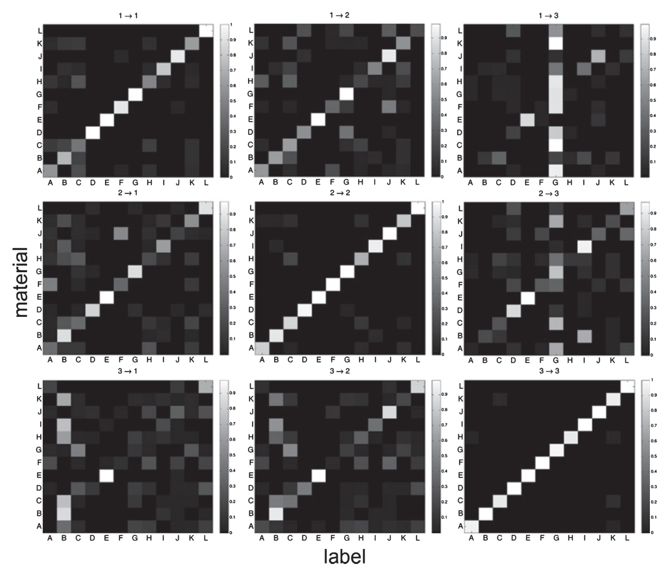
图 12 · 群体反应的多变量结构
原文图注:Fig. 12. Population analysis of responses of IT neurons to images of 12 materials illuminated from each of three different directions. (A) Tree diagram of the results of a cluster analysis based on the correlation of the normalized responses to the 36 original images. The three different illumination directions are indicated by different colors (red, blue and black corresponding to 22.5°, 45.0° and 67.5°, respectively) and numbers (as in Fig. 2A). The letters indicate the 12 materials using the convention of Fig. 1A ('e' is the lettuce leaf). Horizontal stippled lines and the numbers indicate the three different clusters. (B) Scree plot of the principal component analysis of the same data as employed in a showing the eigenvalues as a function of the PC number. The per cent explained variances for the first four PCs are indicated at the corresponding data points. (C and D) Results of the PCA of the same data as that employed in A. Same color and letter conventions as in A. (C) Plot of factor coordinates of the 36 images on PC1 and PC2. (D) Plot of factor coordinates of the 36 images on PC1 and PC3. Per cent explained variance for each PC is listed on the abscissa and ordinate legends. Cluster 1, 2 and 3 of the Cluster Analysis (A) can also be seen in the results of the PCA analysis: cluster 2 corresponds to the three images of the lettuce leaf, which are positioned in the upper right corner of plot D, cluster 3 is differentiated from cluster 1 along PC2, with the images of cluster 1 positioned in the upper left corner of plot C.
基于归一化反应相关矩阵的聚类树与 PCA:36 张原图聚成三簇——16 张七种材料的低仰角图像、三张生菜叶图像、其余图像;PC1 解释 45% 方差,主要区分生菜叶与其余,PC2(9%)区分第一簇与第三簇。这张图界定了后文 PC1/PC2 语义解读的基础,支撑结果第 5 条。
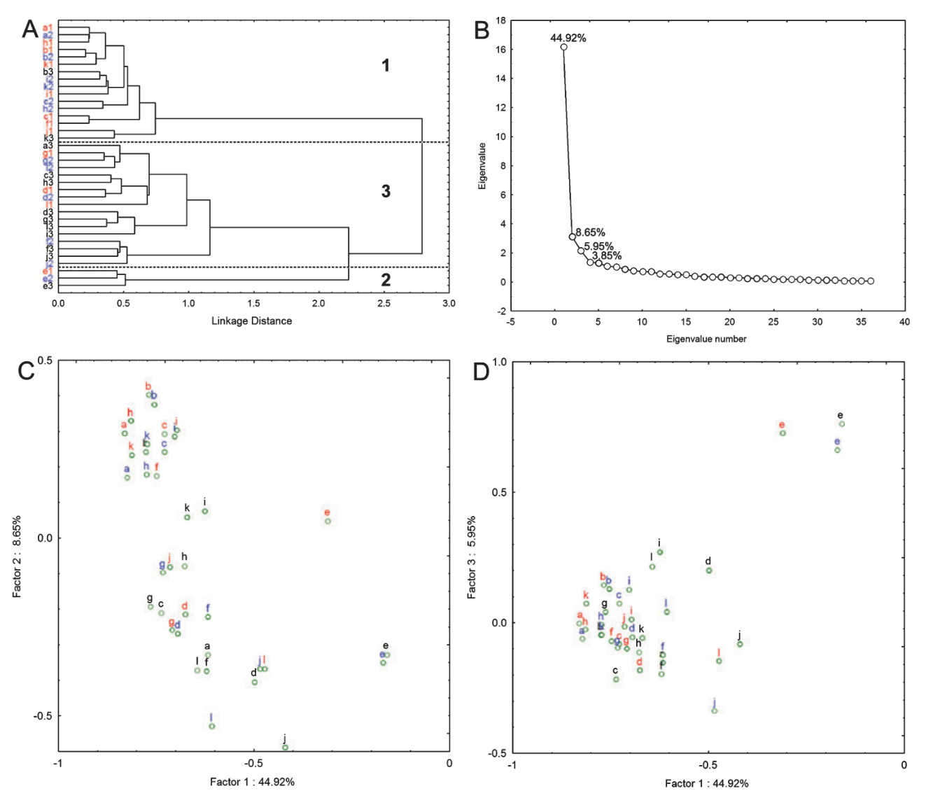
图 13 · 原图与随机相位图响应的 PCA 对比
原文图注:Fig. 13. Principal components analysis of the responses to the original and random phase images. (A) Principal components analysis of the normalized responses to the 36 original (closed symbols) and 36 random phase (open symbols) images. (B) Principal components analysis of the normalized responses to the 33 original (closed symbols) and the corresponding 33 random phase (open symbols) images, thus excluding responses to the three lettuce leaf images. The letters and numbers indicate the material (as in Fig. 1A) and the illumination directions (as in Fig. 2A), respectively. The image coordinates for the first two principal components are shown.
把 72 张图(原图实心、相位图空心)投到 PC1–PC2 平面:沿 PC1 方向原图与相位图明显分居两处(生菜叶与第三簇中如此),而 PC2 上两实心—空心点几乎成对重合。B 面板剔除生菜叶后 PC1 分离依旧存在(解释 53% 方差),排除了"生菜叶特殊性"的解释。这是结果第 5 条的核心证据图。
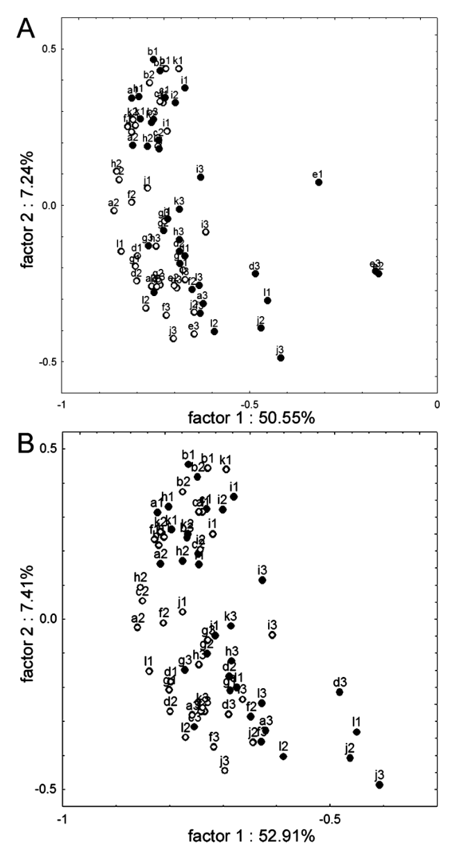
图 14 · 原图与相位图主成分坐标的相关
原文图注:Fig. 14. Correlation of principal component coordinates of the 36 original images and their corresponding random phase images. (A) PC1 coordinates. (B) PC2 coordinates. Stippled and solid lines indicate the diagonal and linear regression fit, respectively.
横轴为原图坐标、纵轴为对应相位图坐标,虚线为对角线(完全一致)、实线为回归拟合。A 图 PC1 坐标只有弱相关(r=0.48)且系统偏离对角线,B 图 PC2 坐标紧密贴合对角线(r=0.90)。一图概括"PC1 相位相关、PC2 功率谱相关"的双分量结论。
讨论
作者从四个方面总结讨论了实验结果:
- 材质编码与经验依赖:IT 神经元对真实材质图像表现出选择性响应,表明高级视觉皮层参与材质信息的表征。作者区分了“特定材质识别”与“跨变换材质归类”:后者要求神经系统对多种图像变体中的共性特征敏感,而本研究中动物仅执行注视任务、未接受材质分类训练,可能限制了更高级抽象表征的展现。
- 光照敏感性与知觉恒常性:相比于人类被试表现出的光照无关分类,IT 单细胞对光照方向变化敏感,跨光照条件的响应不变性有限(平均响应波动 1.5–1.7 倍)。作者指出,缺乏场景全局光照语境线索可能部分影响了恒常性表现;同时单细胞不变性不足与群体层面可成功跨光照线性解码(SVM 正确率显著高于偶然水平)并存,反映了分布式群体编码的容错特征。
- 空间相位与高阶统计特性:主成分分析显示,亮度与功率谱参数仅解释不到 10% 的神经方差,解释约 45% 方差的 PC1 显著依赖图像的空间相位结构。这表明材料纹理选择性主要受边缘、对比度极性与局部结构等高阶图像统计特征驱动,而非低阶空间频率功率谱调谐。
- 形状与材质的可分离表征:双调谐细胞的乘法可分离模型拟合良好(S=0.81),提示形状轮廓与表面材质在很大程度上作为独立特征维度处理。这与人类功能成像中外侧枕区(LO)在轮廓与纹理任务中均被激活但腹侧/内侧区域呈现功能分化的观察相契合。作者同时承认实验局限:每种材质在每个光照方向仅有一张正对视角照片,且生菜叶等样本带有明显的内部叶脉形状特征(剔除生菜叶后核心统计结论依然保持)。
一句话总结
该文在猕猴下颞叶证实了材质纹理与物体轮廓的相对独立编码,发现单神经元材质偏好受光照方向显著调制,而群体反应仍携带跨光照的材质线性可分信息,且该选择性依赖图像的高阶空间相位结构。