High baseline activity in inferior temporal cortex improves neural and behavioral discriminability during visual categorization

这篇文章用清醒猕猴的单细胞记录，把"刺激出现前的基线活动（baseline activity）"和随后的诱发反应、以及猴子在身体/非身体分类任务中的对错联系起来，串出了一条完整的神经事件链：低频（<8 Hz）节律性基线振荡 → 伽马功率与基线放电升高 → 诱发反应选择性与可靠性提升 → 神经分类器与行为表现变好。它值得读，是因为把人类脑成像里"刺激前状态预测知觉"的经典发现，第一次在高级视觉区单神经元水平上和行为直接挂钩，并尖锐地提醒大家：常规分析里"基线校正"这个默认动作，可能一直在扔掉重要的信号。

研究背景

神经元在没有感觉输入时也会自发放电（spontaneous firing），这种基线活动长期以来被视为背景噪声。但到了 2000 年代，一系列人类研究开始颠覆这个看法：fMRI 发现基线活动水平能预测行为表现（如 Ress 等 2000、Hesselmann 等 2008），EEG/MEG 则发现刺激前振荡的功率和相位与知觉成败相关（如 Busch 等 2009）。也就是说，大脑在"看见"之前处于什么状态，部分决定了这次能不能看见。然而这些人类影像研究无法触及单神经元层面：基线放电水平与行为到底有什么关系、其背后的振荡机制是什么，都没有直接证据；而且"振荡的功率"和"放电水平的高低"这两个各自独立被研究的现象之间是什么关系，在当时也是空白的。

作者选择猕猴下颞叶皮层（inferior temporal cortex, IT）作为切入点有明确理由。IT 是腹侧视觉通路的最后一站，神经元对身体、面孔等物体类别有强选择性，团队此前还用微刺激证明 IT 活动对类别知觉有因果影响（Afraz 等 2006）。同时 IT 受注意、预期等自上而下信号强烈调制，而这些认知因素恰恰可能通过自上而下的反馈改变刺激前状态。所以在这个区域做"基线活动—诱发反应—行为"三者关系的考察，既有类别编码的便利，又有承接认知调制机制的意义。缺口在于：单神经元水平上，基线活动如何与诱发反应交互、进而影响神经编码与行为，此前无人系统回答。

研究思路

作者的总体策略是"先分状态、再追链条"。第一步先把试次按刺激前的基线放电水平分成高基线试次（high baseline trials, HBT）与低基线试次（low baseline trials, LBT），看行为对错与基线高低是否相关；第二步问这个"基线高低"在振荡结构上意味着什么——用自协变函数（auto-covariation）和时频分析检查 HBT/LBT 之间的低频节律、相位锁定与伽马功率差异；第三步检验基线状态是否改变了诱发反应的幅度、选择性（身体 vs 非身体的反应差）和变异性（Fano 因子）；最后用线性分类器评估神经群体可分性，并直接对比 HBT/LBT 中的行为 d′。这条逻辑链的巧妙之处在于每个环节都是相邻的因果候选：振荡→放电水平→反应质量→决策，最后再用"前一试次发生了什么"（Fig 7）和"眼动"（Fig 8）两个对照排除混淆，把基线状态定性为一种内生的、类似"脑状态"的东西而非任务事件的残留。

方法

被试为两只成年雄性猕猴（9 岁与 8 岁），在无菌条件下植入头部固定装置与记录舱。任务是二选一强迫选择的身体/非身体分类：猴子先注视中央点一段可变时长（350/400/450 ms，故意不确定以模拟自然情境），随后呈现 70 ms 的 7°×7° 灰度照片，经过 500 ms 空屏后出现左右两个选择目标，猴子需在 300 ms 内扫视到对应目标。刺激共 720 张带噪照片（身体类含人、猴、四足动物；非身体类含飞机、汽车、椅子，各 90 张），每张分四个信号水平（90/70/55/40% 信号），另有 90 张全噪声图（随机奖励 50%，不计入神经分析）。用钨丝微电极在 STS 下岸、TEp 与 TEa 的网格位置上做胞外单细胞记录，共 61 个记录 session、123 个有视觉反应的单细胞（猴 1 贡献 49 个、猴 2 贡献 74 个），其中用选择性指数（selectivity index, SI）判定出 75 个"身体神经元"进入主要分析。

分析窗口以刺激出现为 0：基线取 −200–0 ms（部分时频分析用 −300–0 ms），诱发取 150–350 ms。核心指标包括：区分对错试次反应幅度的正确/错误指数（correct/wrong index, CWI）、HBT/LBT 的自协变函数及其 FFT 幅谱、小波时频功率、相位锁定因子（phase-locking factor, PLF）、以 theta 谷点为基准的尖峰概率与伽马功率对齐（考察交叉频率耦合）、速率匹配的 Fano 因子（Fano factor，衡量反应变异性，要求 65 个神经元满足速率匹配标准）、以及在线性支持向量机（support vector machine）上用 150–350 ms 诱发反应做身体/非身体解码（75% 训练、25% 测试，重复 1000 次）。行为端用信号检测论的 d′（dprime）量化。改为：低频频谱、相位锁定及部分眼动分析采用置换检验；差分反应、速率匹配 Fano 因子和行为 d′ 采用 t 检验。非偏好类别的 Fano 因子仅呈下降趋势，未达到 P<0.05。

主要结果

1. 基线放电水平预测行为对错：身体神经元在基线期（−200–0 ms，平均 7.2±0.7 Hz）的放电率在正确试次中显著高于错误试次，群体基线 CWI 为 9.2±2%（P<10⁻⁵，图 2C）；且基线 CWI 与神经元类别选择性强弱正相关（Pearson r=0.54，P<10⁻⁵，图 2D），即越"专职"的身体神经元，其基线状态对行为的预示作用越明显。

2. 高基线对应强低频振荡：按基线放电分组后，HBT 的自协变函数呈现明显低频振荡而 LBT 几乎没有，FFT 显示 2–7 Hz 频段（与 delta/theta 带重叠）HBT 幅度显著更大（置换检验 P<0.001，图 3）；时频分析确认 <8 Hz 功率差集中在基线期，在诱发反应起始（约 100 ms）附近消失（图 4A–C）。HBT 的低频振荡还相位锁定于刺激出现（PLF 差异 P<0.001，图 4D），并同时伴随基线期伽马（30–90 Hz）功率升高（P<0.001）。

3. 低频相位组织放电与跨频耦合：以 theta 谷点对齐可见尖峰概率的周期性起伏（图 4E），且 theta 谷点与低伽马（<50 Hz）功率存在交叉频率耦合（cross-frequency coupling，图 4F），提示低频节律为放电提供了一个周期性的高兴奋性时间窗。

4. 基线状态提升诱发反应的质量：诱发反应本身在正确试次中更高（诱发 CWI=8.4±1.7%，P<10⁻⁵，图 5A），且与 SI 正相关（r=0.36，P=0.0006，图 5B）；逐试次看，44% 的身体神经元基线与诱发放电率显著正相关，群体平均相关系数 0.124±0.0173（P<10⁻⁵，图 5C）。更重要的是，HBT 中身体/非身体的差分反应显著更大（Δresponse=0.027±0.014，P=0.03，图 6A），速率匹配后的 Fano 因子显著更低（偏好类别 ΔFF=−0.06±0.02，P=0.01；非偏好类别 −0.04±0.029，P=0.06，图 6B）——放电率提升是有类别偏好的（增益式），而变异性下降则不挑类别。

5. 神经与行为表现同步受益：线性分类器在 HBT 试次中的解码准确率比 LBT 高 3.5±0.6%（P<10⁻⁵，图 6C）；行为 d′ 同样显著更高（Δd′=0.04±0.02，P=0.016，图 6D）。对照分析显示前一试次的图像类别、噪声水平、猴子的选择与对错都不影响下一试次基线（图 7 各面板 P 值 0.16–0.7），HBT/LBT 之间眼动功率谱与微扫视频次也无差异（图 8，P>0.05），排除了主要混淆。

图注解读

图 1 · 任务范式、行为表现与记录位置

原文图注：FIGURE 1 | Experimental paradigm and behavioral results. (A) Monkeys were trained to perform a two-alternative forced-choice body/non-body categorization task. The stimulus set contained 720 photographs of body and non-body images, in four different signal levels, and 90 full-noise stimuli. For illustration only, stimulus is depicted here with a relatively large size compared to the monitor screen. Numbers represent the duration of each epoch. (B) Monkeys' performance. Images on the X-axis are examples of noisy stimuli in different signal levels. The error bars represent the ±1 standard error of the mean (s.e.m.) across recording sessions (n = 61). (C) Sagittal section of the MRI at the anteroposterior level of 16 in monkey 1. Red lines depict the boundaries of recording area (lower bank of STS and TE). White vertical line schematically represents the inserted electrode.

这张图是全篇的舞台说明。(A) 给出试次时序：注视（350–450 ms）→ 70 ms 图像 → 500 ms 延迟 → 左右两个扫视目标，刺激集为 720 张四档噪声照片加 90 张全噪声图；(B) 是以"选择身体的百分比"画出的心理物理曲线，信号越强表现越好，全噪声时两只猴子都接近 50%（47.6% 与 48.3%），只有轻微的非身体偏好；(C) 用 MRI 矢状面标出记录区域（STS 下岸与 TE）。它支撑的是"行为任务有效、记录位置可信"这一前提，也是后文所有百分比与 d′ 的出处。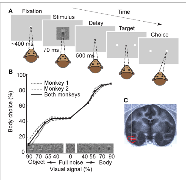

图 2 · 基线放电在对错试次间的差异

原文图注：FIGURE 2 | Modulation of baseline activity in correct vs. wrong trials. (A,B) Normalized firing rate in correct and wrong trials, in a representative body neuron (C36, selectivity index = 0.15) (A), and across all neurons (B). In each neuron and each signal level, the peak response was measured separately in correct and wrong trials. The larger peak was selected to normalize both correct and wrong trials. Finally the normalized firing rates were averaged across noise levels. The gray boxes represent periods of baseline and evoked activity used for the further analysis. In (B) shaded areas represent s.e.m. of correct and wrong responses across the population. The line above the X-axis represents the significant difference between correct and wrong responses, obtained by paired t-test in 50-ms sliding windows with 1-ms steps, plotted at the middle of each bin (t-test, alpha = 0.05). Stimuli were presented for 70 ms, represented by a black bar on the X-axis. (C) Histogram of the CWI (correct/wrong index) in the baseline period. (D) The relationship of baseline CWI with the selectivity index.

读法：(A)(B) 是以刺激出现为 0 的归一化放电率曲线，绿/红（正确/错误）两条线在刺激出现之前的灰色基线窗内就已分开，(B) 中横轴上方的标记给出滑窗 t 检验的显著时段；(C) 把每个神经元的基线 CWI 画成直方图，分布整体偏正（均值 9.2±2%）；(D) 的散点表明 CWI 越大的神经元选择性指数越高（r=0.54）。这张图直接支撑结果第 1 条：刺激还没出现，对错已经"写"在基线放电里了。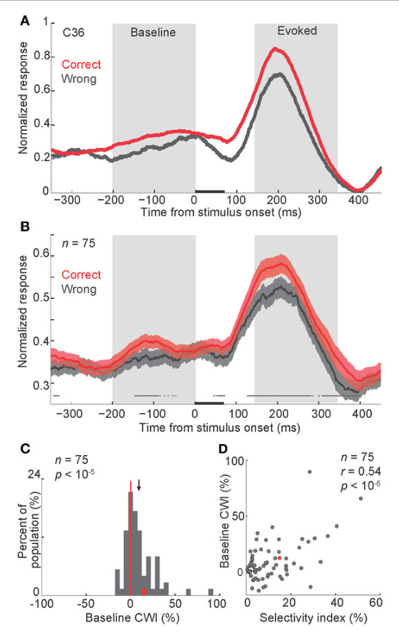

图 3 · 高/低基线试次的振荡结构

原文图注：FIGURE 3 | Oscillation associated with different levels of baseline activity. (A) The auto-covariation plot for high baseline trials (HBT) and low baseline trials (LBT), measured during the baseline period (−300–0 ms). Low auto-covariation within 2 ms of the central time bin reflects the absolute refractory period of the isolated single units. (B) The FFT amplitude of the auto-covariation in HBT and LBT.

(A) 是尖峰序列的自协变函数：中心 2 ms 内的低谷对应单单元的不应期（确认分离质量），而 HBT 在数百毫秒尺度上呈现起伏的周期结构，LBT 则平坦；(B) 把 (A) 做 FFT，可见 HBT 在 2–7 Hz（delta/theta 范围）幅度明显高于 LBT（置换检验 P<0.001）。它支撑结果第 2 条的前半句：基线放电的高低不是均匀的速率差，而是"有没有节律"的质别。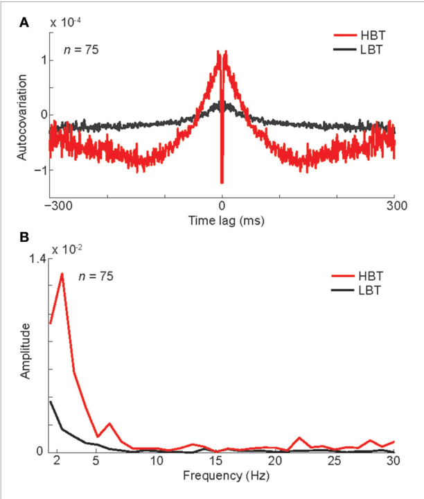

图 4 · 基线状态的频谱、相位与跨频耦合

原文图注：FIGURE 4 | Spectral power and phase associated with different levels of baseline activity. (A,B) The averaged spectral power of the population of body neurons in HBT (A), and LBT (B). (C) The difference of the spectral power in HBT vs. LBT. (D) The difference of the phase locking in HBT compared to LBT. (E) Coupling between the theta troughs and the spike probability. (F) Coupling between the theta troughs and the gamma power.

(A)(B) 是 HBT/LBT 各自的时频功率图（时间×频率），(C) 是二者之差，可见显著的正差集中在 <8 Hz 且位于基线期，诱发反应起始后消失；(D) 的 PLF 差值图说明 HBT 的低频相位在刺激出现前后都是跨试次对齐的；(E) 以 theta 谷点为 0 对齐的尖峰概率呈多个峰，(F) 则显示 theta 谷点后伽马功率周期性升高。这一整张图把"振荡→放电概率→伽马"的机制细节铺开，支撑结果第 2、3 条。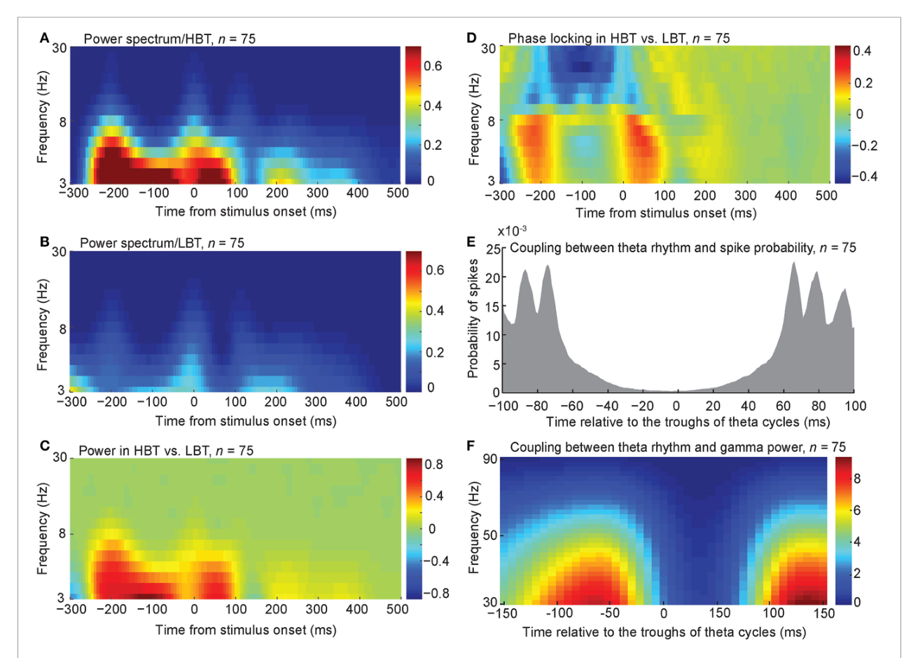

图 5 · 诱发反应的对错调制与基线—诱发相关

原文图注：FIGURE 5 | Modulation of the evoked response in correct vs. wrong trials; correlation of baseline and evoked responses. (A) Histogram of the CWI of the evoked response. (B) The relationship of the evoked CWI with the selectivity index. (C) The histogram representing the correlation of baseline and evoked firing rate. Each data point shows the correlation coefficient value for one body neuron.

(A) 是诱发窗（150–350 ms）CWI 的直方图，群体均值 8.4±1.7%，显著为正，且与基线 CWI 无显著差异（P=0.37）；(B) 显示诱发 CWI 也随选择性指数升高（r=0.36）；(C) 中每个点是一个神经元的逐试次基线—诱发相关系数，44% 显著为正、群体均值 0.124。这张图把"对错差异"从基线期延伸到诱发期，并给出二者逐试次联动的证据，支撑结果第 4 条的第一半。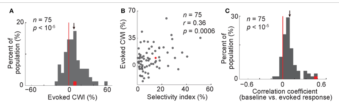

图 6 · 基线状态对神经与行为判别力的贡献

原文图注：FIGURE 6 | Contribution of the baseline activity to the evoked response, neural and behavioral performance. (A) The histogram showing the modulation of the differential neural responses in HBT vs. LBT. This differential response (Δresponse) was obtained by subtracting the normalized evoked response to non-body images from the normalized evoked response to body images. One data point (X = 0.91) was larger than the X-axis limit and is not shown here (B) The modulation of the rate-matched Fano factor in HBT vs. LBT. (C) The performance of a neural classifier in HBT and LBT. Error bars indicate the s.e.m. over 1000 repetitions of the classification in each condition. (D) The modulation of the behavioral dprime (d′) in HBT vs. LBT.

四个面板分别是：HBT−LBT 的差分反应直方图（均值 +0.027，显著为正，图 6A）、速率匹配后 Fano 因子之差（偏好类别 −0.06，显著为负，图 6B）、分类器在两种状态下的准确率（HBT 高 3.5±0.6%，图 6C）、以及行为 d′ 之差（+0.04，P=0.016，图 6D）。这是全篇的"收益总账"：基线状态同时改善信号（判别力）与噪声（变异性），并兑现为神经与行为两个层面的绩效提升，支撑结果第 4、5 条。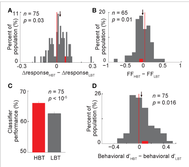

图 7 · 前一试次事件不影响下一试次基线

原文图注：FIGURE 7 | Relationship between different events in the preceding trial and the baseline firing rate in the following trial. The baseline firing rates were compared between different conditions of the last trial: a body or a non-body image was presented (A), a high-noise (90 and 70%) or low-noise (55 and 40%) image was presented (B), a body or a non-body choice was made by the monkey (C), a correct or a wrong choice was made by the monkey (D). Each data point shows the one body neuron.

四个散点图分别按前一试次的图像类别、噪声水平、猴子的选择方向和对错分组比较下一试次的基线放电率，全部无显著差异（P=0.7、0.2、0.16、0.4）。这张对照图的意义是否定性的：基线状态不是前一试次任何可辨识事件的直接残留，更像一种内生的脑状态，支撑结果第 5 条之后的对照部分。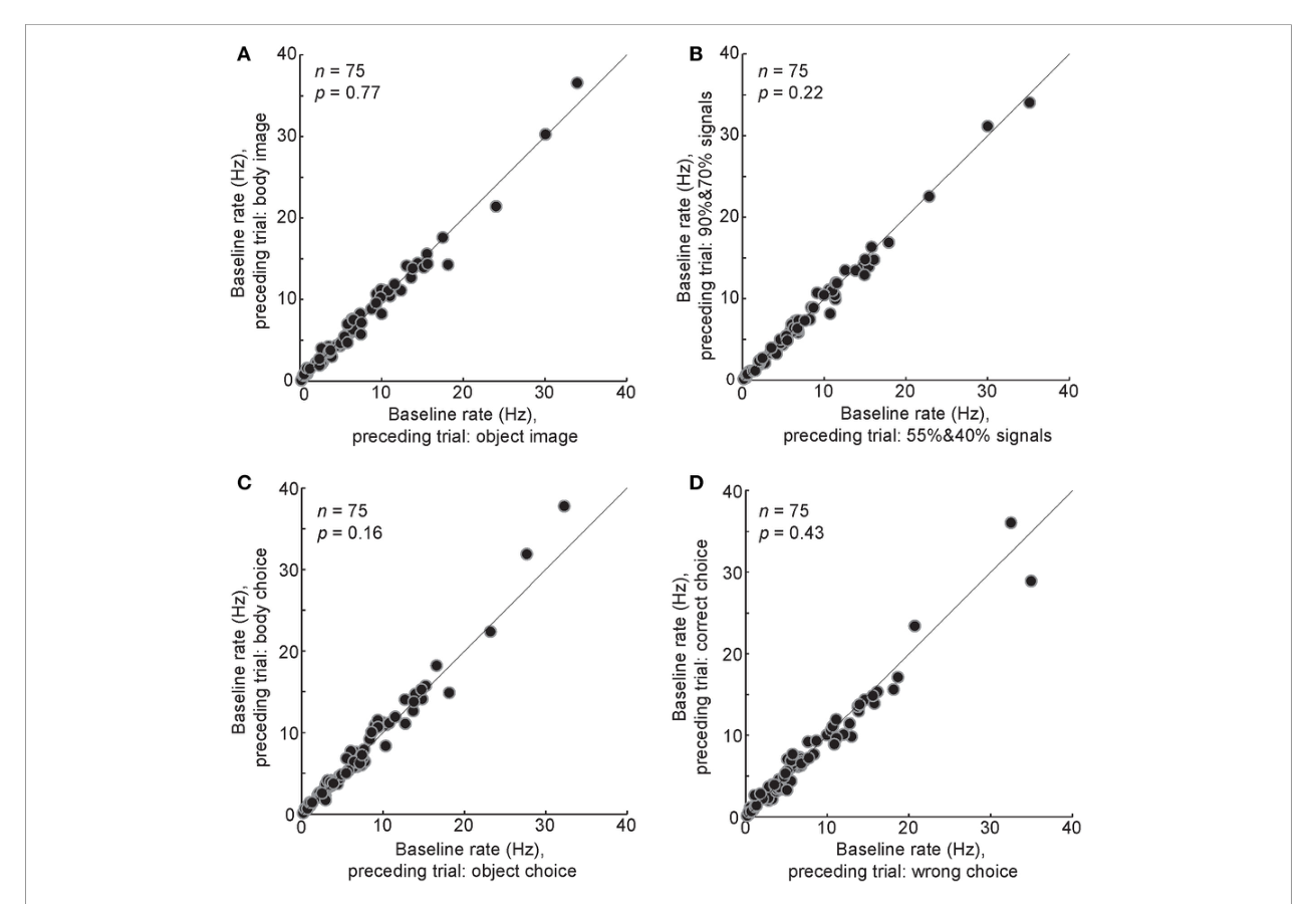

图 8 · 眼动对照

原文图注：FIGURE 8 | Monkeys' eye movements in HBT and LBT. The power spectrum of the monkeys' horizontal (X) and vertical (Y) eye positions in single trials, during baseline period (−300–0 ms), is shown. To test if the results were different between HBT and LBT we performed a permutation test, separately for horizontal and vertical positions. In the permutation test, the trials were randomly assigned to HBT and LBT while keeping the number of trials in each condition unchanged. We compared the experimental spectral power difference with the distribution of spectral power differences obtained from 1000 such permutations. The results showed that the difference between the spectral power of HBT vs. the spectral power of LBT, for the horizontal or vertical positions, was not significant (P > 0.05).

这张图检查注视窗内微小眼动（microsaccades）是否是基线差异的来源：水平与垂直眼位在基线期（−300–0 ms）的功率谱在 HBT/LBT 间无差异（置换检验 P>0.05），微扫视次数也几乎相同（1.29 vs 1.33 次，P=0.67）。它支撑结果的对照部分：基线效应不能被眼动解释。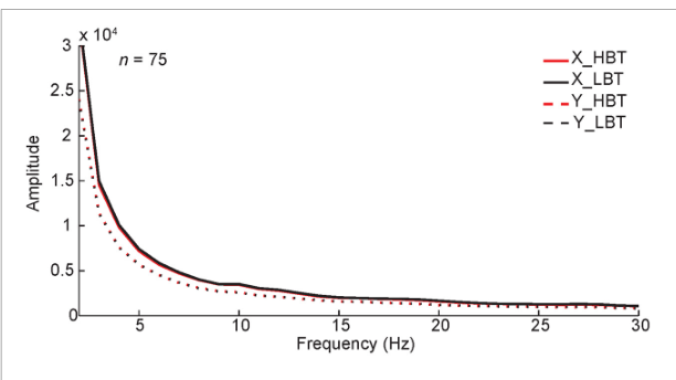

图 9 · 全链条示意模型

原文图注：FIGURE 9 | Neural events following baseline modulation during a categorization task. (A) Schematic diagram of the mean response of a model body neuron responding to body and non-body images in "correct" trials. The impact of rhythmic baseline modulation on the neural response and behavior is illustrated. X-axis as in (B). (B) Plot of normalized averaged firing rate of body neurons in correct trials. In each neuron and each signal level, the firing rates were normalized by the peak response, and then the normalized firing rates were averaged. (C) Schematic diagram of the mean response of a model body neuron responding to body and non-body images in "wrong" trials. The impact of no baseline activity on the neural response and behavior is illustrated. X-axis as in (D). (D) Plot of normalized averaged firing rate of body neurons in wrong trials.

(A)(C) 是模型示意图：有节律基线调制的试次中，振荡的波峰恰好在刺激出现前形成"基线前移"（baseline shift），随后另一个波峰落在刺激期，放大诱发反应并拉开两类反应的分布，使决策边界清晰；(B)(D) 则是正确/错误试次的真实群体平均曲线，形态与模型吻合。这张图是全篇叙事的收束，把前六张图的证据组织成一个"状态决定编码质量、编码质量决定行为"的因果故事。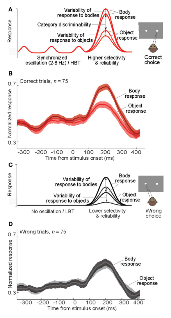

讨论

作者把发现总结为一条五环节的因果链：低频（<8 Hz）振荡出现 → 相位锁定于刺激出现 → 低频与伽马的跨频耦合伴随刺激前的"基线前移" → 神经反应选择性与可靠性提升 → 行为正确。机制上他们给出两层解释：细胞层面，刺激前少数尖峰可提高膜电导、增强反应性（引 Haider 等 2007）；网络层面，节律性基线活动为突触输入的整合提供了精确时间窗（引 Schroeder 与 Lakatos 2009）。他们也提出一个超出"群体同步"经典叙事的单神经元机制：只要每个试次里节律尖峰相对刺激出现的时间一致，单神经元水平的增益就会自动呈现为群体同步。作者承认两个局限：其一，ITT 与前额叶之间是否真有 theta 耦合需要同时记录才能确认（他们引用了 Liebe 等 2012 的 V4–PFC 证据作为旁证）；其二，这是相关证据而非因果，作者明确呼吁用光遗传学在特定时间窗内操纵节律性背景活动来检验因果性。与文献的对话上，文章把脑成像中"刺激前状态"（brain state）与电生理中"注意等认知状态"（cognitive state）两条线索接了起来，并点名批评了电生理分析中普遍用"基线校正"把基线活动从分析中剔除的做法——作者认为这一习惯可能系统性地遮蔽了基线在神经编码中的作用。

一句话总结

按我的理解，这篇文章最大的价值不在于"刺激前活动预测知觉"这个结论本身——人类影像研究早已给出类似图景——而在于它证明这个效应可以从单神经元的振荡结构一路追到行为选择，中间每一环都有数字：改为：低频相位、尖峰概率和低伽马功率之间存在耦合；HBT 同时伴随更强的类别判别和较低的偏好类别反应变异性。这些结果支持候选机制，但不能确定伽马增益或降噪的因果作用。当然相关链条不等于因果，"前一试次事件不解释基线"也只是排除了近端混淆，注意力等内生状态从哪里来文中并未详述；但它至少让"基线校正"从一个无损的预处理步骤变成了一个值得三思的分析决定。