Explicit information for category-orthogonal object properties increases along the ventral stream

这篇文章系统回答了一个常被默认、却很少被正面测量的问题：物体不仅能被被归类，还能被判断位置、大小、姿态——这些"类别正交属性"（category-orthogonal object properties）的信息在腹侧视觉流（ventral visual stream）各层级中是越来越容易提取，还是越来越被丢弃？作者在 V4 与 IT 做大规模阵列电生理记录并辅以 V1 模型，用同一套高变异自然图像跑了十几个解码任务，再以网页心理物理实验拿到人类在同一批图像上的表现作为标尺，最后用只按分类目标训练的层级卷积神经网络（hierarchical convolutional neural network, HCNN）复现了全部规律。结论有力而反直觉：对复杂自然刺激，包括"位置"这种典型低级属性在内，所有类别正交属性的可读出信息都沿腹侧层级增加，而且 IT 的信息格局最能预测人类的行为模式。

研究背景

腹侧视觉流从 V1 经 V4 到 IT（下颞皮层）逐级建立支持不变物体识别的表征，这一点已有大量工作：V1 神经元近似局部边缘检测器，无法在复杂变换下支持类别解码，而 IT 群体活动可直接支持不变分类。相应的观察是"线性分类器能轻松从群体反应中读出类别标签"的信息量沿层级递增——正是这种相邻区域之间可读出信息的相对格局（而非某一区域的绝对隐含信息）约束着可能的神经机制。但视觉系统还要提取大量"类别正交"的属性：位置、尺寸、朝向、三维姿态、长宽比、周长等。这些量常被视为不变识别必须"折扣掉"的杂讯变量（nuisance variables），关于它们的信息如何跨腹侧层级分布，文献给出的印象是零碎的：已知 V1 对简单刺激的位置等属性极度敏感，也已知 IT 保留对位置、姿态的某些信息（DiCarlo & Maunsell 2003、Li et al. 2009 等），但从没有人做过跨区域的系统比较，也没有人把神经解码成绩与人类在同一批图像上的行为水平放进同一坐标。

于是至少有四种定性不同的假说并存（图 1）：H1 主导性的"局部编码"观——层级汇聚以牺牲位置/姿态信息换取不变性，正交属性信息应递减（H1a：早期区域即匹配人类水平；H1b：到 IT 才匹配）；H2：中间区域（类比 V2 边界归属细胞）上信息达到峰值；H3：信息既不丢失也不增益、一路保持；H4：与分类任务一样，正交属性信息也沿层级增加（与粗编码 coarse coding 的思想相容）。哪条曲线是对的，决定了我们对腹侧流乃至"位置信息是否走背侧流"这类多条流假设的判断——这正是缺口。

研究思路

作者的设计是把"一套刺激、多任务、多区域、人类对标"四件事钉在同一个坐标系里。刺激集是刻意挑选的高变异自然图像：同一目标物体在位置、尺寸、三维姿态上大幅变化并叠在杂乱自然场景背景上，从而同时支持类别任务与各种类别正交估计任务。表征能力用"线性可读出信息"（linearly accessible information）量化——线性支持向量机与 L2 正则化线性回归分别对应离散与连续任务，这既是负责任的保守估计，也是对下游神经元的合理速率码模型。区域对比包括实测的 V4 与 IT 群体、仿 V1 的 Gabor 小波模型与像素基线；人类表现用同样的图像在众包平台上测量，然后回答两个问题：各区域要多少个位点才能达到人类水平？哪个区域的跨任务表现格局预测人类行为格局最好？再往下挖信息在位点间的分布与任务间的重叠，最后问：一个只为分类训练、从未见过任何正交属性监督 HCNN，能否自发产生同样的跨层级信息格局。

方法

神经数据来自两只清醒固视的雄性恒河猴（7 与 9 kg），改为『九片 96 电极阵列跨两只猴的三个半球（两左一右，每半球三片），覆盖 V4、后/中/前 IT』。，共 392 个视觉驱动位点（IT 266、V4 126）。刺激以 RSVP（快速序列视觉呈现：每张 100 ms 图像、间隔 100 ms 灰屏）呈现，物体中心在注视点周围 8° 半径内变化，重复记录每图 25–50 次，反应取呈现后 70–170 ms 的棘波计数（扣除背景、按 block 方差归一）——这个早期时间窗以自下而上前馈为主。图像集含 5,760 张：8 个类别（动物、船、车、椅、脸、水果、飞机、桌）各 8 个具体型号（如 BMW 325），高变异条件定义为位置偏移至多一个物体尺度（|h|,|v|≤0.6）、尺度 0.625–1.6、三个轴 ±90° 旋转。任务电池 16 个：基础级 8 类分类、下位级型号识别（8 类各一个 8 选 1 任务合并计），加水平/垂直位置、包围盒宽高与面积、二维视网膜面积、周长、三维尺度、主轴长度与角度、长宽比、x/y/z 三维转角等连续估计任务。解码在留出图像上做交叉验证（80/20，50 次划分），离散任务用平衡准确率、连续任务用预测值与真值的 Pearson 相关。人类数据用 Amazon Mechanical Turk 收集，每任务约 80 人，先 10 个训练试次（带正确答案反馈）再 100 个测试试次（样图呈现 100 ms），组内信度 0.69–0.97。达到人类平价所需的位点数由性能-位点数曲线的 log-线性外推估计；跨任务行为一致性用人类表现向量与神经/模型表现向量之间的 Spearman 等级相关衡量。另有系列对照：V4 与 IT 位点的跨试次信度（0.73 vs 0.76）、选择性与图像对可分性均无或仅有临界差异，感受野覆盖（V4 约中心 4°、IT 约 8°）限制到中心 4° 后结果不变，多单元与分拣出的单单元（IT 154、V4 191 个）模式一致。

主要结果

1. 高变异图像上信息沿层级一致增加（图 3）：16 个任务全部如此——IT 群体的线性解码性能显著高于 V4（多数任务 P<0.005），且差距比单最佳位点更大；IT 在所有任务上优于 V1 模型，V4 在多数任务上也如此；像素控制几乎垫底。单位点层面，多数任务的最佳 IT 位点也显著强于最佳 V4 位点。因此连"位置"这种被认为最"低级"的属性，在 IT 里也最清晰地显式编码。
2. IT 群体用不到几千个位点就够到人类水平，V4 则差几个数量级（图 4 与表 1）：跨任务平均 IT 需 695±142 个位点（均 <2,000）即可达到人类中位表现；V4 往往需要十的六次方以上（基础分类 2.2×10⁶、下位识别 4.4×10⁶；明确写为『对 V4（及 V1/像素），z/x 轴转角所需位点数外推超过 10¹⁰（表 1 以 – 标记）；IT 分别为 1,932±1,061 与 1,570±530』，并统一数量级表述。），长宽比是唯一 V4 接近 IT 的任务（951±59 vs 163±61）。按单试次单神经元换算，中位数 695 个重复平均的多单元位点约对应 8.3 万个 IT 神经元。
3. 跨任务难度格局由 IT 决定：把 14 个任务的人类表现向量与各群体表现向量做 Spearman 相关（图 4b,c），IT 显著最一致（更细的按类别拆分出的 41 个点同样支持），一次 ANOVA 显示四组群体的一致性差异 p<10⁻⁵（F=164.52）。这提示 IT（而非 V4/V1）更直接驱动下游行为。
4. 信息广布而非专设（图 5）：以 107 个解码器的权重分布分析，每个任务的"高权重"位点占全部位点的 15–35%（均值 26.3%），与同规模高斯分布（32.5%）相比，接近半数任务的稀疏度不可区分——没有任务专属的专家单元群。任务两两重叠（权重向量绝对值的相关）56.5% 为正、高重叠集中在语义相关任务组；唯一的例外是面孔检测任务，其与其他任务的重叠显著低于随机水平（P<0.01）——恰与已知的面孔模块现象吻合，也为这套重叠度量提供了阳性对照。总体上，IT 对类别与非类别任务是联合编码。
5. 只优化分类的模型自发复现全部格局（图 6）：一个六隐藏层 HCNN 在 ImageNet 上仅以类别标签训练（剔除与测试集重叠的类别），各层在每个任务上的性能随层级单调上升（呼应图 3）；训练过程中，顶层对非类别任务的估计精度随测试集分类性能同步爬升（图 6b,c）——即使其输出层被显式训练成对这些参数"不变"。训练后的顶层信息格局与 IT 高度一致且逐层趋近（图 6d,e）。
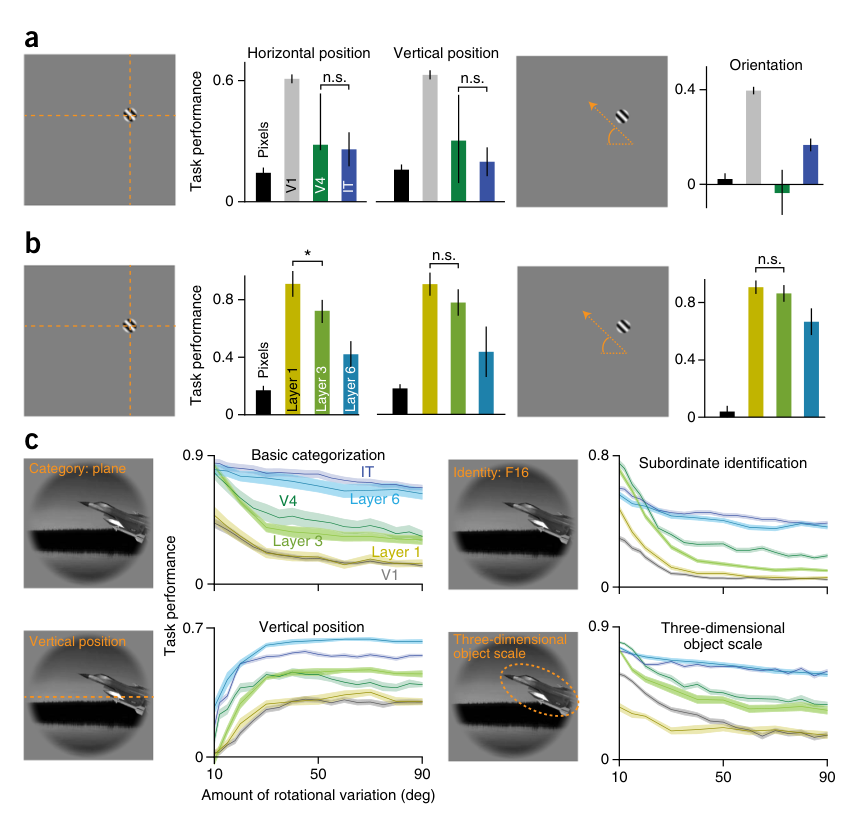
6. 变异量而非任务类型是决定因素（图 7）：改为『在位置任务上 IT 不再优于 V4（朝向任务差异亦不显著），且 V4 与 IT 均逊于 V1 模型』；模型第 1 层最高、越高越低。把高变异集按旋转变异（10°–90°）取子集，随变异减小 V4-IT 差距收窄（16 个任务中 13 个在 P<0.005 显著），个别任务（下位识别、三维尺度）甚至反超；而用低变异合成集训练的替代模型复现不出高变异模型的信息格局。

图注解读

图 1 · 四种假说的图解

原文图注：Figure 1 Illustration of possible scenarios. (a) Prior to this study, extensive research has shown that invariant category recognition performance increases along the ventral pathway (top), whereas lower and intermediate visual areas are sensitive to various categorical-orthogonal properties (position, border continuity, etc.) in simple stimuli. It was also known that IT contains some information for category-orthogonal properties: as illustrated (bottom), performance in IT must be above floor. (b) However, the previous literature determined neither the relative amounts of explicitly decodable information for category-orthogonal properties between ventral cortical areas nor the ratio of neural decode performance in IT (or elsewhere) to measured behavioral performance levels. In other words, there were multiple qualitatively different hypotheses consistent with the known data as to both the red curve's shape and its height on the y axis. In hypothesis H1a, there is a tradeoff between increasing receptive field size and categorization ability, and performance on the orthogonal task. Early areas match human performance on these tasks, whereas later areas do not. This is probably the dominant view in the visual neuroscience community. In hypothesis H1b, the same tradeoff holds as in H1a, except that the human performance is matched in IT, rather than early layers. In hypothesis H2, explicitly decodable information peaks (for at least some non-categorical properties) in intermediate visual areas, analogous with the results for V2 border-ownership cells that have been found in the context of simple visual stimuli. In hypothesis H3, information is neither lost nor gained for the orthogonal variable tasks up through the ventral stream, it is simply preserved. This view is suggested as one possibility in previous studies from our group and is consistent with ideas of hyperacuity. Finally, in hypothesis H4, information increases for the orthogonal tasks along with the categorization tasks. Aspects of this possibility are consistent with coarse coding.

解读：上排画的是已知事实（分类信息递增；低级区对简单刺激的正交属性敏感；IT 至少有"高于地板"的一些信息），下排画的是五种候选曲线——H1a/H1b 都主张递减（差别只在何处达到人类水平），H2 主张中间区峰值，H3 主张水平保持，H4 主张与分类同向上升。红色曲线即"类别正交性能随腹侧层级深度"的走向，纵轴以人类水平为 1。这张图界定了全文要裁决的问题空间；正文图 3 显示只有 H4 在复杂刺激上成立。

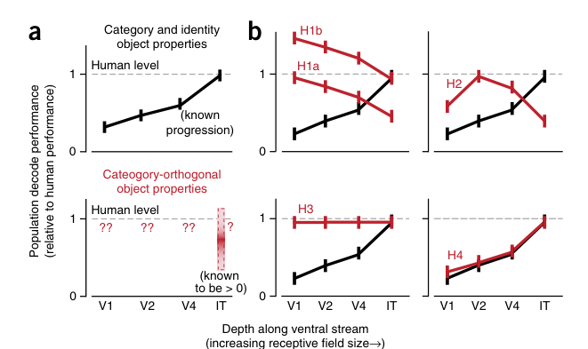
图 2 · 刺激、记录与解码流水线

原文图注：Figure 2 Large-scale electrophysiological measurement of neural responses in macaque IT and V4 cortex to visual object stimuli containing high levels of object viewpoint variation. (a) We recorded neural responses to 5,760 high-variation naturalistic images consisting of 64 exemplar objects in eight categories (animals, boats, cars, chairs, faces, fruits, planes, tables), placed on natural scene backgrounds, at a wide range of positions, sizes and poses. (b) Stimuli were presented to awake fixating animals for 100 ms in a rapid serial visual presentation (RSVP) procedure (horizontal black bars indicate stimulus-presentation period). Object centers varied within 8° of fixation center. Recordings were made using chronically implanted electrode arrays, collecting a total of 392 neuronal sites in IT (n = 266) and V4 (n = 126) visual cortex. Each stimulus was repeated between 25 and 50 times. Spike counts were binned in the time window 70–170 ms post stimulus presentation (as indicated by shaded regions) and averaged across repetitions, to produce a 5,760 × 392 neural response pattern array. (c) We then used linear readouts to decode a variety of types of image information from the neural responses, including categorical data such as object category and exemplar identity, as well as continuous data such as object position, retinal and three-dimensional object size, two- and three-dimensional pose angles, object perimeter, and aspect ratio.

解读：三栏分别是刺激集示意（类别、型号、位置/姿态/尺度变异、自然场景背景）、RSVP 时间线与阵列记录（阴影标出 70–170 ms 计数窗），以及群体读出流程：5,760 图 × 392 位的响应矩阵接入线性解码器，输出从分类到位置、尺寸、姿态、周长、长宽比等各种属性。读懂这张图就等于握住了全文的坐标系。

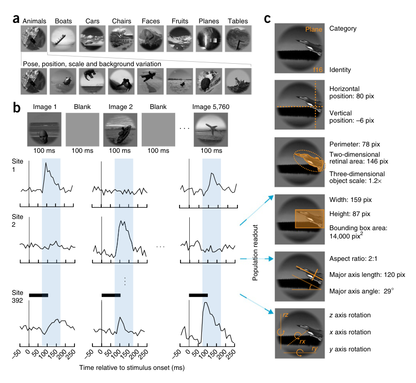
图 3 · 各区域对 16 个任务的解码对比

原文图注：Figure 3 Comparison between ventral cortical areas of object property information encoding in high-variation stimuli. (a) Performance of single best sites from IT (blue bars) and V4 (green bars) on each task measured task. Best sites were chosen in a cross-validated manner, with performance being evaluated on held-out images. Chance performance is at 0. Error bars represent s.d. of the mean taken over subsets of images used to choose the best site for each task. n.s. indicates IT-V4 difference not significant, P < 0.05, P < 0.005. (b) Population decoding. For each task, we trained a linear decoder on neural output. For discrete-valued tasks, including object categorization and subordinate identification, we used support vector machine (SVM) classifiers with L2-regularization. For continuous-valued estimation tasks, we used linear regression with L2-regularization. We compared decoding performance for our recorded IT population sample (blue bars) and V4 population sample (green bars), as well as for a performance-optimized V1 Gabor wavelet model with competitive normalization (gray bars) and the trivial pixel control (black bars). For categorical properties, bar height represents balanced accuracy (0 = chance, 1 = perfect). For continuous properties, bar height represents the Pearson correlation between the predicted value and the actual ground-truth value. All values are shown on cross-validated testing images held out during classifier and regressor training. All evaluations are performed with n = 126 sites and a fixed number of training and testing examples. Error bars represent s.d. of the mean over cross-validation image splits and, in the case of pixel, V1 and IT data, over multiple subsamplings of 126 units from the whole population. In b, IT-V4 and V4-V1 separations were significant at P < 0.005 except where notated; n.s. indicates difference not significant, P < 0.05. See Supplementary Table 1 for statistical details.

解读：a 是逐任务的"最佳单电极"对比（蓝 IT、绿 V4，机遇水平为 0），b 是固定 126 位点的群体解码对比（另加灰色的 V1 模型与黑色的像素基线）。纵轴对离散任务是平衡准确率、对连续任务是预测-真值 Pearson 相关。读图要点：绝大多数任务上蓝柱 > 绿柱 > 灰柱 > 黑柱，IT-V4 差异多标注 P<0.005，只有少数任务（如图中 3D 尺度附近）标 n.s. 或仅 P<0.05。这张图是主要结果第 1 条的直接证据。

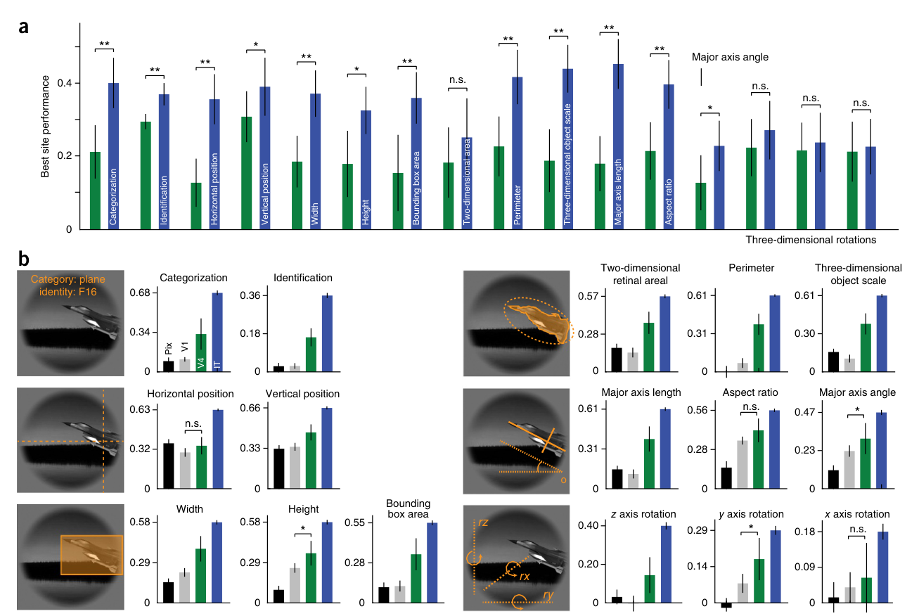
图 4 · 神经解码与人类表现的对标

原文图注：Figure 4 Comparison of neural population decoding performance to human psychophysical measurements. (a) Human-relative performance as a function of number of subsampled sites used to decode the property, for selected tasks. The x axis represents the number of sites. For each task, the y axis represents the performance of the decoder with the indicated number of sites, as a fraction of median human performance for that task, with a value of 1 indicating human performance parity. Decoder performance metrics and training procedures are as described in Figure 3b. Solid lines represent measured data and dotted lines represent log-linear extrapolations based on the measured data. Shaded areas around each solid line represent s.e. assessed by bootstrap resampling of sites and images. We evaluated our measured IT (blue lines) and V4 (green lines) neural populations out to the entire recorded populations of 266 and 126 sites, respectively, and evaluated V1 model (gray lines) and pixels (black lines) out to 2,000 units. Human performance for each indicated task was measured using large-scale web-based psychophysics. 1 s.d. in the human performance is indicated by gray shading flanking y = 1 (median performance level). (b) Scatters show human performance (x axis) versus neural performance (y axis) for a variety of tasks. Large squares (n = 14) correspond to the tasks indicated in Table 1. Small circles (n = 41) indicate values for further breakdown of the data into subordinate identification and pose estimation tasks on a per-category basis. (c) Summary of data from b. Bar height represents Spearman's R correlation between human and neural decode for the aggregated large-square tasks (left) and disaggregated small-circle tasks (right). Error bars are s.d. of the mean due to task and image variation. The dotted line represents the mean self-consistency of the measured human population, averaged across multiple subsets of the population sample. Horizontal gray bars represent the s.d. of the mean of human self-consistency, across population, task and image subsets. n.s. indicates difference not significant, P < 0.05, *P < 0.005. See Supplementary Table 1 for statistical details.

解读：a 是核心曲线——纵轴以人类中位表现为 1，横轴位点数（对数刻度）：IT 蓝线最先撞到 y=1 的"人类平价带"，V4 绿线按外推要数十万甚至更多位点，V1 模型与像素线始终够不到；dotted 线是 log-线性外推。b 把每任务的人类表现（横轴）对神经解码性能（纵轴）画成散点，跨任务走势的匹配度即 c 中的 Spearman R——IT 最高、显著高于 V4/V1/像素。这组图支撑主要结果第 2、3 条，即"多少位点、哪种格局"两层意义上 IT 都最像行为的发生地。

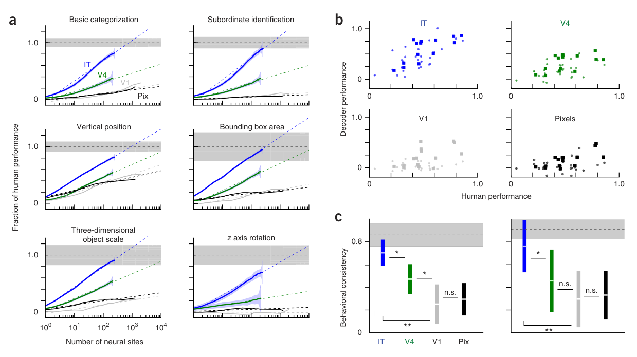
图 5 · 信息在 IT 位点间的分布与任务间重叠

原文图注：Figure 5 Distribution and overlap of IT cortex site contribution across tasks. (a) Histograms of values of sparseness over all tasks. Sparseness is measured via excess kurtosis (γ2). Reference values show fractions of 'high-relevance' sites, as determined by three-point distribution method. Gray band represents 1 s.d. of distribution of sparseness values taken on size-matched samples from a Gaussian distribution. (b) Histograms of values of imbalance over all tasks. Imbalance is measured via skewness (γ1). Reference values at the top of the imbalance panel show fractions of values above versus below means, ranging from 1.3 to 0.7. Gray band represents 1 s.d. of distribution of imbalance values taken on size-matched samples from a Gaussian distribution. (c) Sparseness (left) and imbalance (right) of weight distributions for selected tasks. Error bars represent s.d. over image splits on which weights were determined. Gray bands here are defined as in a and b. (d) Quantification of weight pattern overlap for pairs of tasks. Each colored square in the heat map is the Pearson correlation between the absolute value of the weight vectors for a pair of tasks. A high value (red color) indicates that the weight pattern for the pair of tasks is similar; a low value (blue color) indicates the opposite. White indicates a value that is not statistically significantly different from zero. The order of tasks is the same as in c.

解读：a、b 的直方图看每个任务权重分布的形状——尖峰度（sparseness）衡量"是否只有少数位点被高权重选中"，偏度（imbalance）衡量正相关与负相关位点谁多。多数任务落在同规模高斯样本的灰色带内（高权重位点 15–35%、Gaussian 对照 32.5%），比例接近对称（0.7–1.3），说明没有任务专属的小集团。d 的热图看任务两两重叠：多数格偏红（56.5% 正重叠），语义相近的任务（各类尺寸任务）成块发红，而面孔检测一行/列发蓝色。此图支撑主要结果第 4 条。

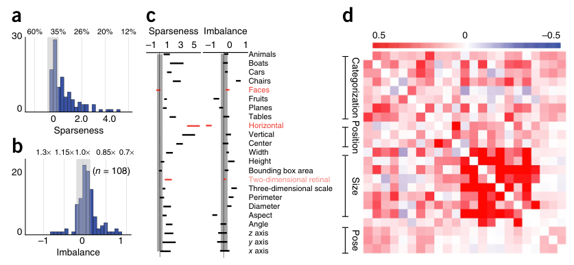
图 6 · 计算模型复现跨层级信息格局

原文图注：Figure 6 Computational modeling results. (a) Performance of fully-trained model at each hidden layer. y axes are as described in Figure 3b for corresponding tasks. (b) Scatter plots of performance of computational model's top hidden layer on training-set categorization performance versus testing-set estimation accuracy for selected non-categorical tasks. Each dot represents a state of the model during training. (c) Quantification of relationship in b, shown for all tested tasks aside from categorization itself (n = 15). Bar height represents Pearson correlation of accuracy on indicated task with test-set categorization performance, taken across training time steps. Error bars represent s.d. of the mean taken across both time steps as well as splits of images used for performance assessment. (d) Scatter plot of performance of top hidden layer of fully trained model versus performance of IT neural representation, on each task measured in Table 1. As in Figure 4b, large squares represent aggregated tasks (n = 16) and small circles represent disaggregated tasks (n = 43). Unlike Figure 4b, several tasks are included for which human data were not collected. (e) Consistency of fully trained model with neural performance pattern across layers, using the same metric described in Figure 4c. y axis and error bars are as described in Figure 4c. See Supplementary Table 1 for statistical details.

解读：a 显示六层模型从浅到深在所有任务上的性能都单调上升；b、c 是训练时程分析——顶层在测试集上对非类别任务的表现随分类表现同步增长（每个点是一个训练时刻的模型快照），意味着"为分类学习而堆出来的表征顺手把位置、姿态都表征了"；d 为模型顶层 vs IT 神经的逐任务散点（大方块 16 个聚合任务、小圈 43 个拆分任务）；e 用与图 4c 相同的一致性指标显示这种吻合随模型层级加深而增强。此图支撑主要结果第 5 条。

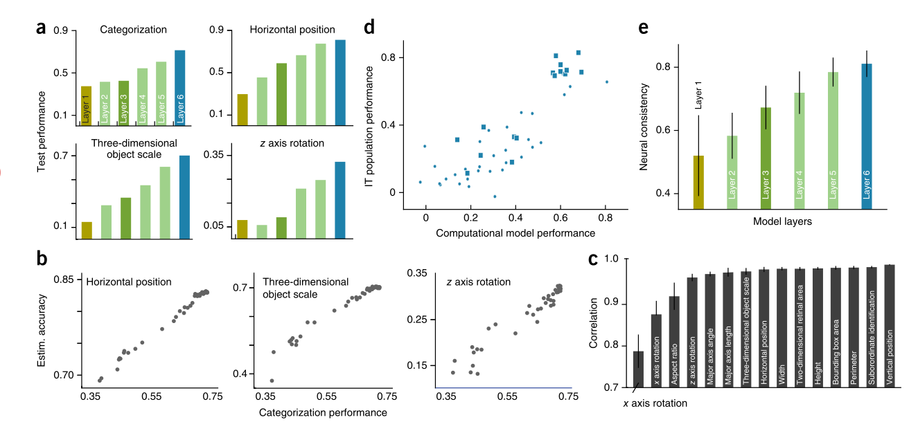
图 7 · 信息格局依赖刺激变异量

原文图注：Figure 7 Dependence of linearly accessible information on the amount of variation in stimuli. (a) Population neural decoding results for position and orientation tasks defined on a simpler stimulus set consisting of grating patches placed on gray backgrounds. y axis, bar colors and error bars are as described in Figure 3b. (b) Performance of three selected neural network model layers (layer 1, yellow; layer 3, olive green; layer 6, cyan) for the tasks shown in a. (c) Population decoding performance as a function of amount of rotational variation in classifier training and testing data sets, for each of several representative object tasks, for measured IT neural population, V4 neural population, V1 model and for the three model layers. x axis represents (absolute value of) the amount of rotational variation allowed in all three rotational axes; for example, a value of 10 corresponds to rotation in x, y and z axes ranging from −10 to 10 degrees. y axis is performance evaluated using the same metrics and decoder training procedures as described in Figure 3b. Error bars are computed over selections of sites and units as well as image training splits (see Supplementary Table 1 for statistical details).

解读：a 用灰底光栅块重复图 3b 式的分析——此时灰色 V1 模型柱反超，V4 与 IT 显著高于机遇但 IT 不再优于 V4；b 显示模型同样的层内倒序（第 1 层最高、第 6 层最低）。c 把训练/测试集按三轴旋转变异量（如 x 轴取 10 即 ±10°）切分：总体上变异越小，V4-IT 与顶层-中层模型差距越小，个别任务甚至反转。此图支撑主要结果第 6 条：跨区域的信息格局由变异复杂度决定，而非任务本身的类型。

讨论

作者把实证结果归纳为一句话：在复杂自然图像域，"所有行为相关的物体属性沿腹侧视觉层级协同提取"（H4），而主流的局部编码/权衡观（H1a/H1b）被否定，H3 也不成立。作者指出，这一格局与分布式粗编码表征的既有理论相容：既然衡量标准是线性读出接口，那么层级汇聚的主题任务并不是逐层丢弃物体变换——模型虽然依赖丢弃信息的汇聚（pooling）操作，但其作用不在于对物体变换的逐层折扣。至于机制问题，作者给出一个 HCNN 式的存在性证明：前馈电路、仅以分类为目标，就足以让粗编码式的联合表征成为最优解；学习稳健的类别选择性"免费"附带了对非类别属性的显式表征——至于反过来是否成立（学几种正交属性是否足以带来分类能力），文中留作开放问题。局限方面，作者列举得很清楚：线性解码器只是下游读出的合理假设而非证明；与更低层级的比较用的是 V1 模型而非实测 V1 神经；刺激限制在注视点周围 8°，不足以评判外周/顶叶式的空间处理；数据采自被动固视动物、解码读的是早期诱发反应，因此前馈效应应当占主导，反馈与注意机制未被排除；多物体场景里的特征捆绑问题（binding problem）超出本文范围。作者还顺带设想：腹侧与背侧流可能都携带重叠属性的表征，差别在空间分辨率——腹侧细而中央偏置、背侧粗而覆盖外周，两者配合支持注视导航与逐快照参数解析。最后，这种表示也可被解读为腹侧流在逆推图像空间的生成模型——IT 输出编码了"重跑渲染器"所需的关键参数。

一句话总结

这篇笔记最大的实惠是它把一个流行直觉翻了个面：层级越深不是丢掉越多"低级信息"，而是把位置、尺寸、姿态连同类别都计算得更干脆——前提是刺激世界的变异足够真实。按我的理解，"变异量决定信息格局"这一条其实是全文最深的部分：它说明任何只见过"摆正的中景物体"的模型（或大脑）都无从逼出这种联合表征，也解释了为什么早期文献合情合理地推出了今天的"常识"。