一句话定位:本文通过对 20,840 张带有前景目标边界标注的自然图像进行色度统计分析,结合清醒猕猴下颞叶皮层(IT)的功能磁共振成像(fMRI)与微电极神经生理记录,检验了物体环境颜色分布规律与腹侧视觉流神经元颜色调谐特性的对应关系。
研究背景
颜色视觉有助于物体的快速检测、辨别与长时记忆,并在计算机视觉分类中充当重要特征。然而在下颞叶皮层物体表征的传统研究中,颜色常被作为低阶感觉控制变量,大量电生理与脑成像实验采用去饱和的灰度图像,皮层功能构筑的解释多聚焦于几何形状、语义类别或视网膜尺寸偏好。自然场景统计学研究虽揭示了自然光照与反射率的非均匀分布,但整幅图像的平均统计量混杂了前景与背景,无法明确特定色度属性是否特异性指向独立的前景物体。
因此,量化颜色是否具备物体指示功能需要分离物体像素与背景像素的色调、彩度及亮度对比度分布。若物体与背景存在统计差异,需进一步检验该差异能否支持计算层面的目标二分类,以及“动物/非动物”(animacy)等高级语义分类是否伴随系统性的底层颜色线索。若忽视这些低阶感觉协变量,高级皮层的表征几何可能被过度拟合为纯粹的抽象语义组织。最后,需在统一的视后色度空间中,将图像统计先验与灵长类 IT 皮层的神经群体颜色调谐直接对比,检验皮层表征与自然环境统计之间是否存在解剖层次上的匹配。
Rosenthal 等人建立了包含大规模图像统计、机器学习分类与非人灵长类神经记录的验证链。研究分析了包含显著物体标注的图像库中各颜色属于物体的后验概率,测试了基于纯颜色特征的分类器表现,并测定了猕猴 IT 颜色偏置区的神经调谐特性。需要指出的是,标注图像集来源于人工摄影与特定筛选流程,边界标注亦包含主观判定,且神经调谐相关性不能等同于颜色在识别中的直接因果驱动,相关演化假说仍属待检验推论。
研究思路
研究设计包含三个阶段。第一阶段,量化自然物体的颜色统计特性:基于微软 MSRA 图像数据库中人工筛选的 20,840 张包含显著前景物体的照片,由实验不知情的观察者在边界框内精细提取物体掩膜(产生 2,781 个物体标签并分类为动物性与非动物性两大类),分别计算自然色物体、人工色物体及背景像素在 CIELUV 空间的色调(hue)、彩度(chroma)及 Michelson 亮度对比度分布。
第二阶段,评估颜色信息的分类有效性:以色度特征构建支持向量机(SVM)分类器,测试其区分物体/背景以及动物/非动物图像的准确率,并与基于方向梯度直方图(HOG)的形状特征及 AlexNet 深度卷积网络特征的表现对比。
第三阶段,检验皮层颜色调谐与环境统计的匹配性:利用 12 种在视锥拮抗空间等亮度平面上均匀采样的颜色刺激两只清醒猕猴,测定全脑 fMRI 激活;逐体素计算神经调谐曲线与物体颜色后验概率之间的相关系数;继而在 fMRI 定位的颜色偏置斑块内实施微电极电生理记录,在单单元和多单元水平验证群体调谐特征。
方法
图像数据分析:像素颜色在 CIELUV 色度坐标(u′v′)下表征(图 2 与图 3 采用 D65 白点,其余采用 D50 白点),彩度依据 CIE 1976 标准计算,亮度对比度采用 Michelson 对比度公式。像素色度经 CIECAM02 转换矩阵映射至 LMS 视锥细胞兴奋空间。“物体颜色概率”定义为:在全部图像中,特定颜色出现在物体像素内的频次占该颜色在物体与背景中总出现频次的比例。
猕猴 fMRI 实验:采用 3T Siemens 磁共振扫描仪与专用 AC88 梯度线圈,配合 MION 铁氧化物对比剂采集两只清醒注视猕猴的脑图像(各向同性体素 1 mm³)。视觉刺激包含在视锥拮抗空间等亮度面上定义的 12 种颜色(均等 CIELUV 彩度,平均亮度 55 cd/m²),以色度与灰色交替的漂移光栅形式按区组设计呈现(每区组 32 s),提取各体素的时间序列百分比信号变化(psc)。
微电极电生理记录:包含两组数据:一是在 fMRI 定位的下颞叶后部外侧颜色偏置区(PLc)开展微电极记录(记录猴 M1 的 117 个神经元,涵盖 54 次穿刺),测试 16 种颜色的感受野闪烁刺激放电率;二是提取此前发表的 V4 复合体内颜色小团(globs,N = 300)与团间区(interglobs,N = 181)的电生理数据。刺激为呈现于感受野内的色块(持续 200 ms,灰屏间隔 200 ms,单色至少重复 3 次),计算神经元群体的平均放电率。
主要结果
- 物体与背景的色度分布系统性分离。统计表明,背景像素偏向冷色调(偏蓝、偏绿、低彩度),而物体像素系统性偏向暖色调(偏黄、偏红),这一现象在自然色与人工色物体中均一致存在。区分物体与背景的主要轴向对应 CIE u′ 维度(反映视网膜后级 L-M 视锥拮抗机制),天然物体与背景在 u′ 维度上的差异显著(100 次迭代重采样 t 检验均为 p = 0,v′ 维度 p < 10⁻⁶⁷,图 1)。
- 物体概率与暖色偏移呈正相关。像素统计显示,物体颜色概率与色度 u′(偏暖程度)存在显著正相关:天然物体全像素 r = 0.93,人工物体全像素 r = 0.88;在每幅图像仅随机抽取一对像素的子抽样控制检验中,相关仍稳定存在(天然物体 r = 0.79,人工物体 r = 0.51;两组相关系数差异 Fisher z′ = 5.8,p = 10⁻⁹,图 2)。在彩度方面,物体显著高于背景(最高彩度区间 p = 10⁻¹²),人工着色物体在彩度分布两端均呈现增多现象(图 3)。
- 纯颜色特征可有效实现前景–背景二分类。使用单个像素颜色训练的 SVM 分类器,仅依赖色调维度的分类准确率为 64.5%,依赖彩度为 60.2%,依赖亮度为 48.2%,三特征联合准确率达 65.1%;受试者工作特征曲线下面积(AUC)联合特征为 0.77,色调为 0.72,彩度为 0.63,亮度为 0.63(均 p < 0.0001)。以视锥机制维度测试时,单独的 L、M、S 视锥兴奋度分类能力接近随机猜测水平(49–51%),而 L-M 机制轴准确率达 68.1%(AUC = 0.72),显著优于 S-(L+M) 机制轴的 50.9%(AUC = 0.61,图 4),表明红绿视锥拮抗信号构成了物体检测的关键特征。
- 颜色特征包含动物性分类线索。动物性(animate)与非动物性(inanimate)物体像素的色度分布存在稳定分化,主要体现在 CIE v′(蓝–黄)维度上(100 次重采样迭代中,v′ 维度 100% 达到 p < 10⁻⁸⁰,u′ 维度 77% 达到 p < 0.05,图 5)。对 Kriegeskorte 等人(2008)提出的 92 张标准测试图像,仅输入物体区域的平均 CIE u′v′ 色度坐标,径向基函数(RBF)核 SVM 分类器对动物性物体的判别准确率达 91.67%,对非动物性物体达 70.45%(整体准确率 81.5%,图 6)。在 MSRA 全集上,仅输入色调特征的 SVM 对动物性识别准确率为 76.0%(AUC = 0.70),性能接近基于复杂梯度的 HOG 形状特征(图 6、表 1)。
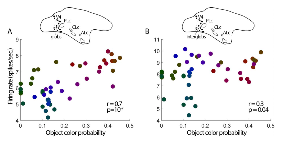
- IT 皮层神经调谐与自然物体颜色统计对齐。fMRI 测定显示,IT 内三个离散的颜色偏置区(后外侧 PLc、中外侧 CLc、前外侧 ALc)均对高物体颜色概率的刺激呈现更强的神经激活(PLc: r = 0.7, p = 0.01;CLc: r = 0.72, p = 0.01;ALc: r = 0.65, p = 0.03,图 7)。全脑逐体素相关图谱显示,该相关性沿着 IT 腹外侧皮层形成宽阔带状分布,IT 区域的平均相关强度显著高于初级视觉皮层 V1(配对 t 检验 p = 0.03);在 PLc 内的微电极单单元记录进一步确认了神经元群体放电率与物体颜色概率的正相关性(r = 0.56, p = 0.025,图 8)。在 V4 复合体内,颜色小团(globs)细胞群体的调谐与物体颜色统计显著相关(r = 0.7, p = 10⁻⁷),其相关性显著高于小团间区(interglobs)神经元(r = 0.3, p = 0.04;群体间差异 Fisher z′ = 2.2, p = 0.02,图 9)。
图注解读
图 1 · 物体像素与背景像素的色度统计对比
原文图注:Figure 1. The color statistics of objects. (A) From over 200,000 images, observers at Microsoft selected 20,840 images that contained a salient object and placed a red bounding box around the object (Liu et al., 2007). Two naïve observers in the present study then created masks to demarcate the pixels containing the object. The top panels show example images; the bottom panels show the masks. (B) Tapestry plots showing 10,000 pixels randomly selected from the pixels assigned to backgrounds (1.89 billon pixels total), naturally colored objects (0.26 billion pixels), and artificially colored objects (0.22 billion pixels). (C) Chromaticity coordinates of the pixel colors of the tapestry plots. The figure shows a single lightness plane through the chromaticity space, with pixels of all lightness projected onto that plane. …… Pixels from naturally colored objects were different from pixels in backgrounds along the u′ dimension (p = 0 for all 100 iterations, unpaired t test), and along the v′ direction (p < 10⁻⁶⁷ for all 100 iterations).
(A) 图像样本及像素掩膜构建流程;(B) 背景像素、天然色物体像素及人工色物体像素各随机抽取 10,000 个构成的织锦分布图;(C) 像素投影至 CIELUV (u′v′) 色度平面的散点分布,内嵌放大数据显示物体像素整体相对于背景像素在 u′(暖色轴)方向发生系统性偏移(100 次独立重采样中,u′ 维度独立样本 t 检验 p 值均等于 0,v′ 维度 p < 10⁻⁶⁷)。
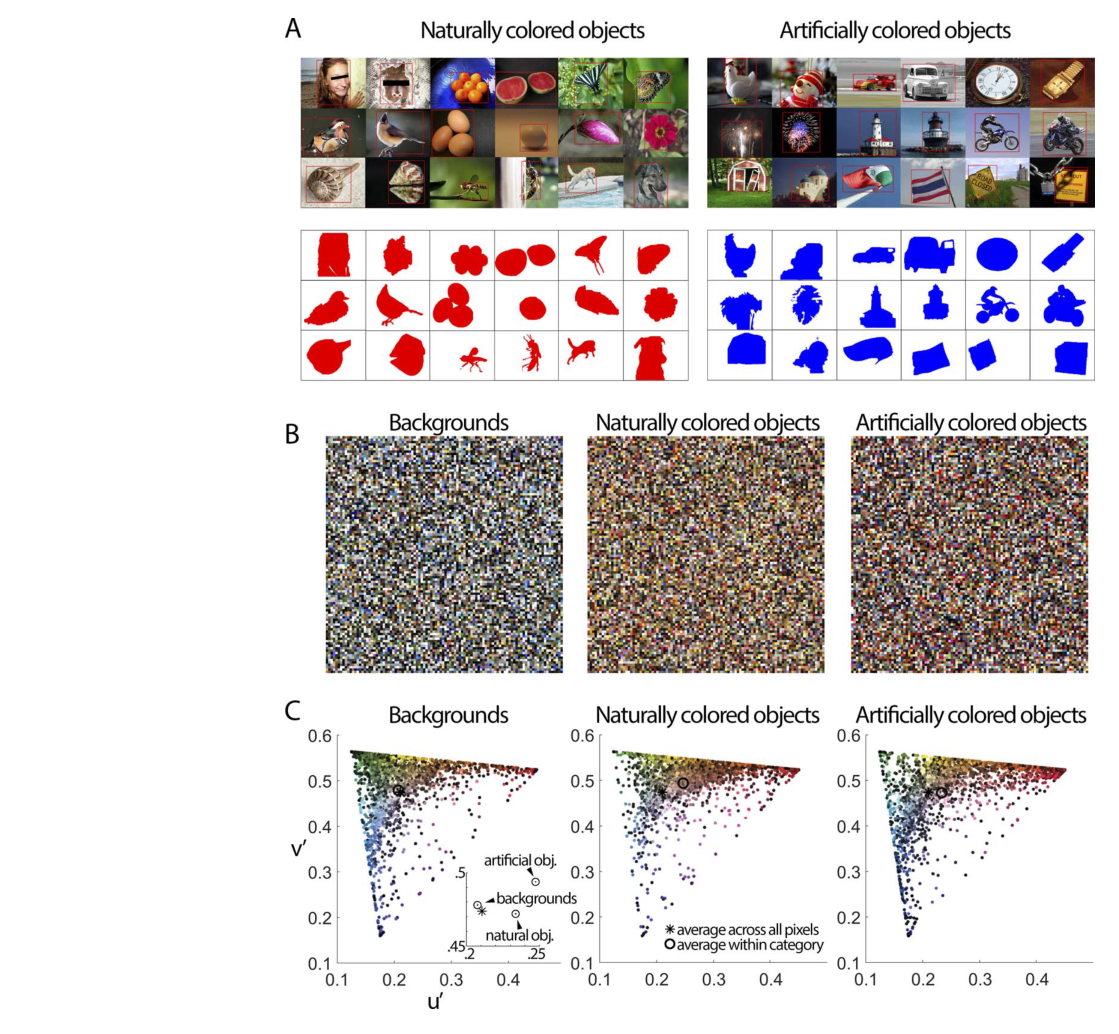
图 2 · 物体颜色概率随暖色程度单调上升
原文图注:Figure 2. Object-color probability, rank-ordered by most frequent object colors. (A) Pixels across the 20,840 images were categorized into 240 bins (24 evenly spaced hue angles at 10 chroma values in u′v′). Object-color probability was computed as follows: number of pixels having a given color in the objects divided by the number of pixels having the same color in the objects + backgrounds. The colors of the bars correspond to the sRGB colors of the bins. The bars are rank-ordered with the most frequently occurring object colors on the left.
(A) 色度空间等间隔划分为 240 个色调×彩度区间,柱高表示该颜色属于物体的后验概率,柱身对应其实际 sRGB 色彩,按概率降序排列(误差线表示 1,000 次 Bootstrap 标准差);(B) 每幅图像仅配对抽取一个前景像素和一个背景像素的控制分析;(C) 物体颜色概率随 u′ 色度坐标变化的散点相关图(箭头指示中性白点),左侧为全样本分析,右侧为单像素对采样,展示出天然物体(r = 0.93)及人工物体(r = 0.88)随暖色程度增加概率递增的趋势。
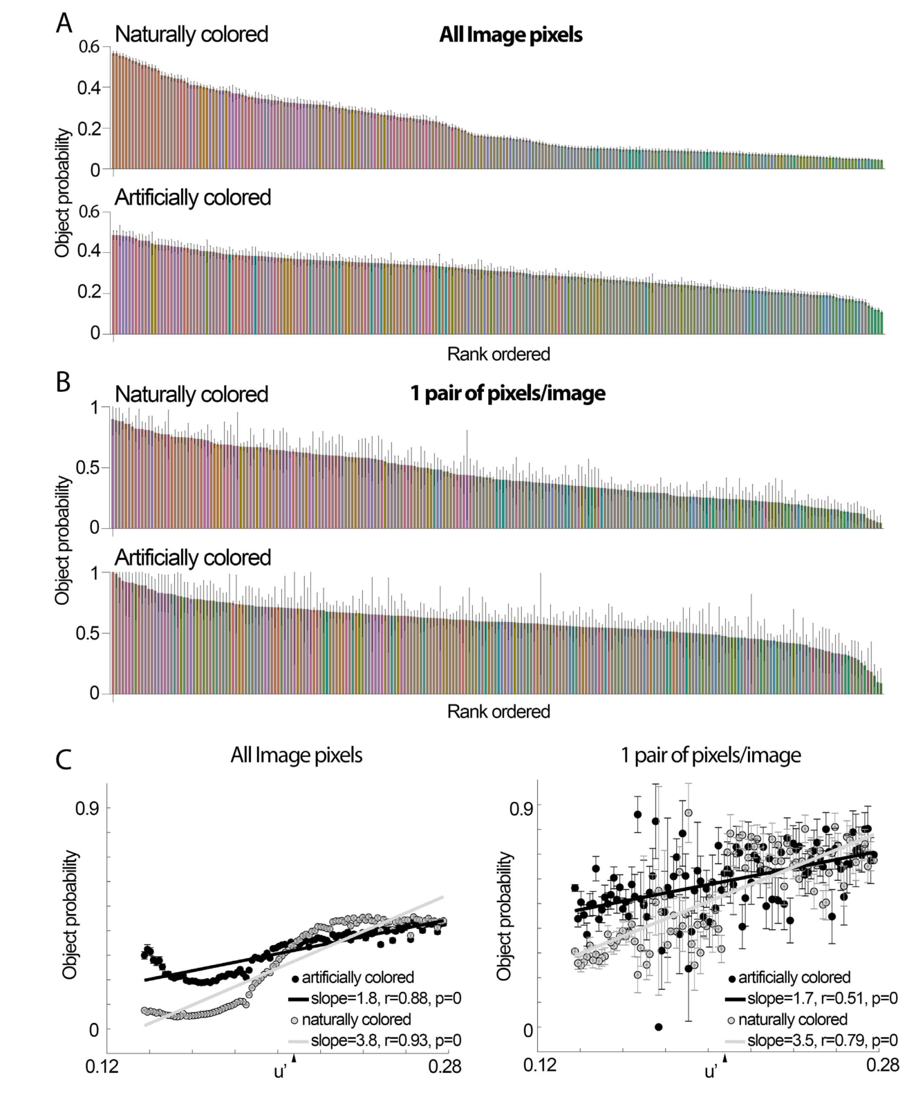
图 3 · 彩度与亮度对比:物体更饱和、人工色走极端
原文图注:Figure 3. Color chroma and luminance-contrast statistics of objects. (A) Histograms showing the chroma of the pixels identified as part of objects (black bars), and the chroma of the pixels identified as part of backgrounds (open bars). Chroma was defined as the CIE 1976 chroma. (B) The chroma of pixels identified as naturally colored (black bars) and artificially colored (open bars). Artificially colored objects were biased towards the chroma extremes, showing more low-chroma pixels and more high-chroma pixels compared to naturally colored objects. (C) The luminance contrast of all image pixels identified as part of naturally colored objects (black bars) are compared against the contrast of the pixels identified as part of artificially colored objects (white bars). …… All differences between pairs of bars identified by an asterisk were significant (chi-square test of proportions, p < 0.03).
(A) 前景物体像素(黑色柱)与背景像素(空心柱)的 CIE 1976 彩度分布直方图,物体在高彩度区间的占比显著偏高(p = 10⁻¹²);(B) 天然色物体与人工色物体的彩度分布对比,人工物体在极低彩度与极高彩度两端均呈现统计富集;(C) 天然色物体与人工色物体的 Michelson 亮度对比度分布对比,星号标明比例检验具有统计学显著性的柱对(卡方检验 p < 0.03)。
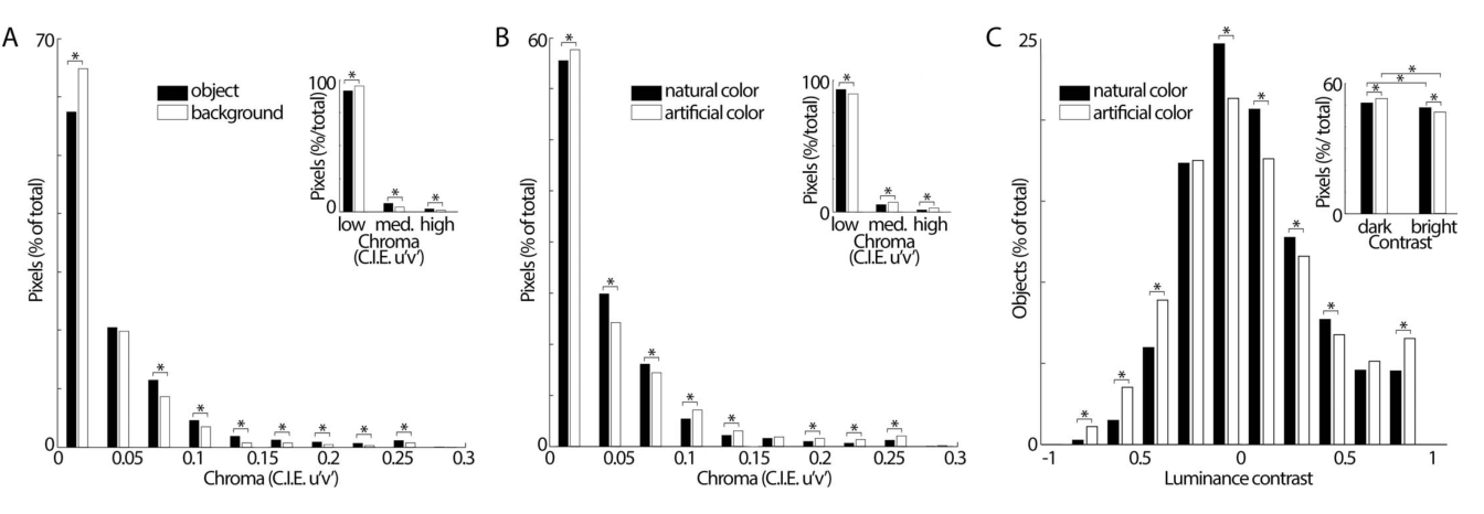
图 4 · 用颜色特征判物体/背景的 ROC 曲线
原文图注:Figure 4. Receiver operating characteristic (ROC) analysis showed that objects can be discriminated from backgrounds based on color. (A) ROC curves when using hue, chroma, and luminance, and all three as input to a support vector machine (SVM) classifier. All ROC curves were significantly different from the null curve (Wilcoxon rank sum test, p < 0.0001). (B) ROC curves when using L, M, S, L-M, S-(L-M), and the two intermediate directions in cone-opponent space as features for SVM for classification (Int1 = orange-blue axis; Int2 = green-purple axis). All ROC curves were different from the null curve (Wilcoxon rank sum test, p < 0.0001). Only the L-M curve and the S curve were different from all other curves, and each other (p < 0.0001).
(A) 基于色调、彩度、亮度单独及三者联合特征分类物体与背景的 ROC 曲线(联合特征 AUC = 0.77,色调 AUC = 0.72);(B) 基于视锥拮抗机制分量的分类性能,L-M 轴(红绿轴)的 ROC 曲线(AUC = 0.72)显著优于 S-(L+M) 轴及孤立视锥输入,证实红绿拮抗维度为区分前景与背景的主要有效特征。
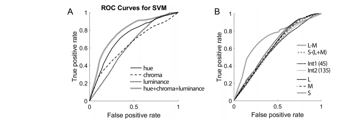
图 5 · 动物与非动物物体的色度统计差异
原文图注:Figure 5. Color statistics differed for animate and inanimate objects. Average chromaticity coordinates for pixels identified as part of animate or inanimate objects. Pixels were drawn from a tapestry of 10,000 randomly selected pixels from each category. This analysis was repeated 100 times. Pixels of animate objects were different from pixels of inanimate objects along the u′ dimension (p < 0.05 for 77/100 iterations), and along the v′ direction (p < 10⁻⁸⁰ for all 100 iterations). Error bars are SEM.
动物性与非动物性物体各抽取 10,000 像素在 CIELUV (u′v′) 平面上的平均色度坐标及 SEM 误差范围。分析重复 100 次,两类物体在 v′(黄蓝轴)维度上表现出高度显著且稳定的分离(100 次重采样均达 p < 10⁻⁸⁰),表明高级生物语义类别与底层黄蓝色度特征存在系统性共变。
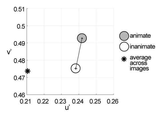
图 6 · 只凭物体平均颜色即可判 animate/inanimate
原文图注:Figure 6. Images could be categorized as animate versus inanimate using only the average color of the object in each image. (A) Chromaticity coordinates for the 92 images used by Kriegestkorte et al. (2008). The asterisks show the neutral point of the color space. The blue circles are the average u′v′ value of all the color values plotted in the figure. (B) A support vector machine with a radial basis function trained on only the average CIE u′v′ of the object in each image categorized animate images at an accuracy of 91.67% and inanimate images at an accuracy of 70.45%. Inset shows the chromaticity coordinates for all images as in A, in which open symbols indicate images classified as "animate" and filled symbols indicated images classified as "inanimate". Stimuli are reproduced with permission from Nico Kriegeskorte.
(A) Kriegeskorte 等人(2008)测试集内 92 张物体的平均 u′v′ 色度分布散点图;(B) 仅依据图像内目标平均色度训练的 RBF 核 SVM 分类结果:动物性物体识别准确率达 91.67%,非动物性达 70.45%。内嵌小图显示模型的决策边界与分类标签分布,表明传统表征相似性分析中识别的“动物性”表征差异可能包含平均颜色特征的贡献。
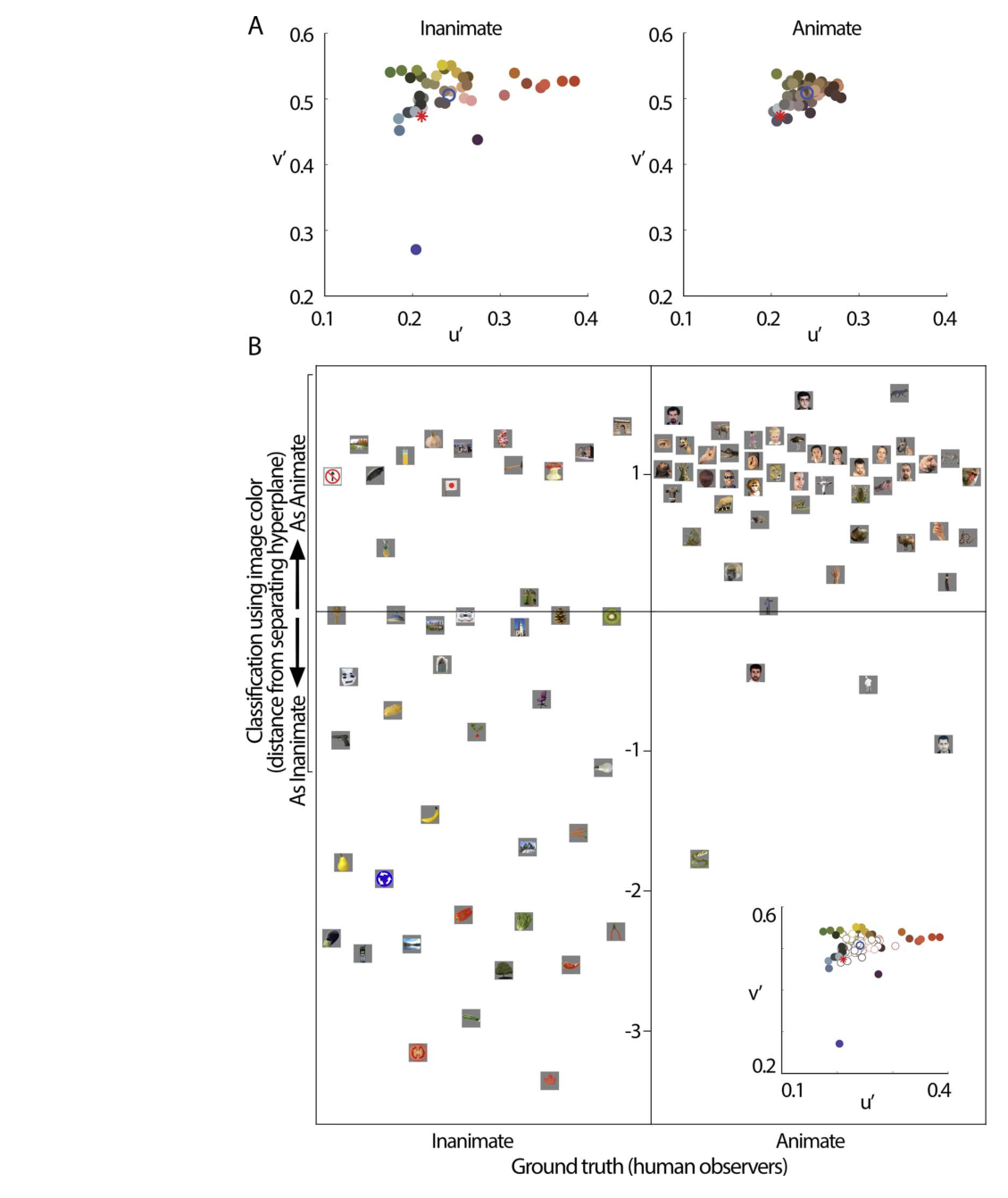
图 7 · IT 三个颜色偏置区的调谐与物体颜色概率正相关
原文图注:Figure 7. Correlation of object-color statistics and color-tuning of IT color-biased regions. A. Diagram of the lateral view of the macaque brain showing the location of the color-biased regions in inferior temporal cortex (IT), anterior is to the right (Posterior Lateral color, PLc; Central Lateral color, CLc; and Anterior lateral color, ALc; Lafer-Sousa & Conway, 2013). (B) Chromaticities of the colors used in these fMRI experiments. (C) Relationship of the probability of object colors versus color-tuning of color-biased regions within IT. Object-color probability was computed as follows: number of pixels having a given color in the objects divided by the number of pixels having the same color in the objects + background, in natural images. All three regions showed higher responses for colors that were more likely to be the colors of objects (PLc: r = 0.7, p = 0.01; CLc: r = 0.72, p = 0.01; ALc: r = 0.65, p = 0.03). fMRI response (psc) = percent signal change.
(A) 猕猴大脑外侧面标明 IT 内三个颜色偏置区(PLc、CLc、ALc)的位置示意;(B) fMRI 测试采用的 12 种等亮度等彩度刺激在色度图中的分布;(C) 三个区域的 fMRI 百分比信号变化随物体颜色概率单调递增,相关系数均具有统计显著性(PLc: r = 0.7; CLc: r = 0.72; ALc: r = 0.65)。
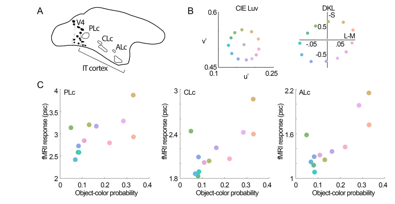
图 8 · 物体颜色概率—颜色调谐相关在全皮层的分布
原文图注:Figure 8. Correlation of object-color statistics across the cerebral cortex. (A) Correlation coefficients between fMRI color tuning and object-color probabilities assessed for each voxel across both hemispheres for one monkey (M1). Color-biased regions are outlined in white; face patches are outlined in black. Vertical meridians are shown as broken lines; horizontal meridians are shown as solid lines. (B) Correlation coefficients were higher in IT compared to V1; the IT region of interest was defined by combining the color-biased regions and the face patches (paired t test across V1 and IT, p = 0.03; LH = left hemisphere; RH = right hemisphere). (C) The population of neurons recorded in fMRI-guided recordings of the posterior color-biased region showed a bias for colors more often associated with objects, consistent with the fMRI results (r = 0.56, p = 0.025). Data were obtained from 117 cells in 54 penetrations in M1.
(A) 猴 M1 双侧半球全脑逐体素相关图谱(白色勾勒颜色偏置区,黑色勾勒面孔斑块),高相关体素集中分布于 IT 皮层带;(B) IT 综合感兴趣区内的平均相关显著高于初级视觉皮层 V1(配对 t 检验 p = 0.03);(C) 基于 fMRI 引导在后部颜色偏置区实施电生理记录,117 个神经元的群体放电率与物体颜色概率显著正相关(r = 0.56, p = 0.025)。
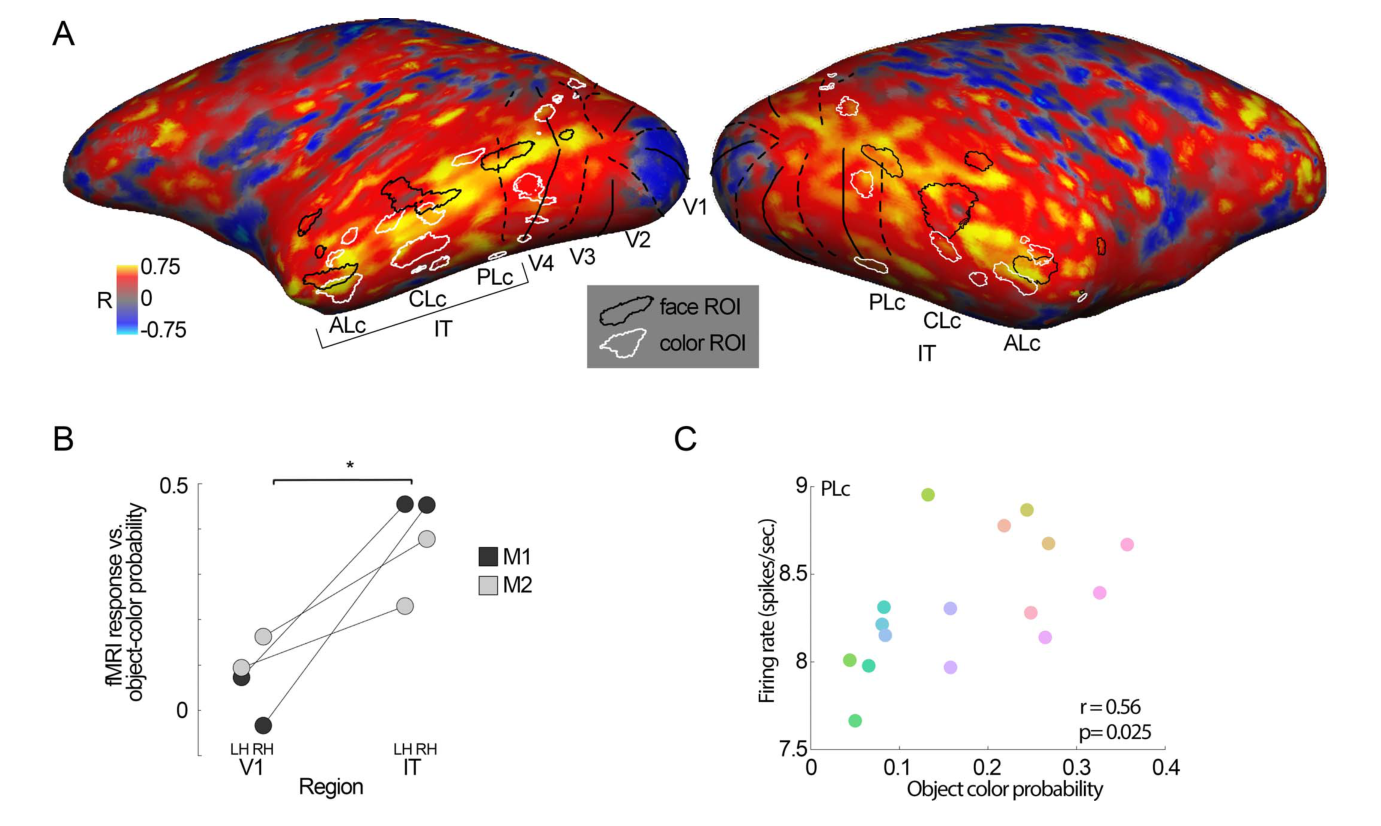
图 9 · globs 与 interglob 细胞群体的调谐—统计相关对比
原文图注:Figure 9. Color-tuning of the population of neurons recorded in posterior IT (the V4 Complex) was correlated with object-color statistics. (A) Responses of cells located within globs (fMRI-identified color-biased regions of the V4 Complex; N = 300 cells. The glob-cell population showed a stronger response to the colors more likely associated with naturally colored objects (r = 0.7, p = 10⁻⁷). (B) Responses of cells located within interglob regions (N = 181 cells). The interglob-cell population showed a stronger response to the colors more likely associated with objects, but a lower correlation coefficient than was found among glob cells (r = 0.3, p = 0.04, Fisher z′ = 2.2, p = 0.02).
(A) V4 复合体内颜色小团(globs,N = 300)神经元群体平均放电率与天然物体颜色概率高度正相关(r = 0.7, p = 10⁻⁷);(B) 小团间区(interglobs,N = 181)神经元群体亦呈现正相关,但相关系数显著低于小团细胞(r = 0.3, p = 0.04;Fisher z′ 变换检验 p = 0.02),表明环境色彩统计的神经表征特异性富集于专门化的颜色功能柱中。
讨论
作者结合实验数据讨论了颜色视觉在视觉场景理解中的功能定位。自然图像中前景物体主要沿 L-M 暖色轴偏移,且偏向较高彩度,这为灵长类三色视觉演化假说提供了环境统计依据:三色视觉可能不仅服务于熟透果实的寻觅,更构成了通用性的前景物体分割机制。颜色信号在此充当了自下而上的显著性线索,引导视觉注意系统分配更高精度的形状辨别计算资源。
针对 IT 皮层的组织模式,实验证明高级视觉皮层的神经调谐曲线特异性匹配了自然物体的颜色分布概率,且这种对齐在层级上呈现自 V1、V4 复合体向 IT 逐级强化的解剖梯度。此外,由于动物性与非动物性物体在 v′ 维度和彩度上存在统计分化,既往以无彩色刺激建立的复杂语义表征模型可能部分吸收了自然界中固有的低阶色彩共变。
研究同时指出若干局限性:MSRA 数据库包含人类摄影者的构图取向与人为筛选偏差,需在无偏差的全景视野数据库中复核;当前生理数据基于两只猕猴的测试,且刺激主要在受控等亮度平面下测量,对于自然界中宽动态范围的明暗变化与三维光影交互仍需进一步深入解析。
一句话总结
本研究证实自然图像中前景物体具有偏向暖色与高彩度的统计特征,且灵长类下颞叶皮层颜色偏置区的神经元群体调谐曲线特异性对应了该环境统计概率,展示了环境先验在高级视觉皮层构筑中的映射。