Representations of regular and irregular shapes by deep convolutional neural networks, monkey inferotemporal neurons and human judgments

一句话定位：这篇文章把一条老牌的猕猴下颞叶（IT, inferior temporal cortex）单细胞形状选择性数据，与深度卷积神经网络（CNN, convolutional neural network）逐层激活、以及人类相似性分组判断放在同一张表现相似性分析（RSA, representational similarity analysis）的桌上比较。结果是：训练过的深层卷积层与 IT 神经元的抽象形状表征高度一致，而人类判断却与更深的全连接层对应更好——层级深度上"猴脑"与"人脑"在 CNN 里的对应点并不相同。

研究背景

近年多项研究显示，深度 CNN 对自然图像的表征与猕猴 IT 反应、人类腹侧通路 fMRI 激活及人类物体识别行为的相关，超过了 HMAX 等既有模型。但这些研究用的都是自然图像——恰好也是训练 CNN 做分类所用的那类图像，存在"用同类图像检验"的循环风险。另一支历史悠久的传统则用二维抽象形状探测 IT 神经元的选择性：Kayaert 等人（2005）曾用一组规则/不规则形状记录了 119 个前 IT 神经元，发现 IT 对规则形状（其差异为非意外属性，NAP, nonaccidental property，即随深度旋转保持不变的性质，如轮廓直或弯、边平行与否）的反应调制大于度量属性（MP, metric property，如长宽比、弯曲程度），且这些差异不能用像素灰度差异或 HMAX C2 表征解释——当时没有任何现成的计算模型能解释这批数据。缺口因此很清楚：CNN 若真是 IT 的现实模型，就必须在"与训练图像性质迥异、却已被证明能驱动 IT 的抽象形状"上也成立，这一泛化此前从未被检验。

研究思路

作者借用 Kayaert 数据集这个"试金石"：形状组之间的像素差异已被刻意平衡（NAP 差异的像素差反而更小），因此任何模型若要匹配 IT 的反应模式，就不能靠低级图像相似性作弊。比较采用二阶同构（second-order isomorphism）逻辑下的 RSA：不重建形状，只问"在 IT 神经空间中彼此靠近的形状，在 CNN 某层激活空间中是否也靠近"。为把"架构本身"与"分类训练"的贡献分开，作者给三个 CNN（Alexnet、VGG-16、VGG-19）各配了一个结构完全相同但权重随机的未训练版本作对照；再把人类对同一形状集的相似性排序数据加进来，检验"人比 IT 更敏感于直/弯对比"这一已知差异会出现在 CNN 的哪一层。另设感受野（RF, receptive field）与形状大小、单元采样比例、主成分（PCA）等三组控制分析，以排除深度效应是感受野增大或少数离群单元驱动的平凡解释。

方法

神经数据沿用 Kayaert 等（2005）：两只雄性恒河猴在被动注视任务下看 64 个形状（约 7°、随机点纹理填充、灰色背景上呈 200 ms），记录窗口为刺激后约 50–150 ms 起的 250 ms 平均放电率，每形状至少 5 次重复（中位 10）；入选的是对形状集有显著选择性（ANOVA, p<0.05）的 119 个前 IT 神经元（猴 1 共 76 个、猴 2 共 43 个），位于上颞沟下岸与前 IT（TEad）外侧凸面。人类数据为 23 名 naive 成人对打印形状做自由分组排序，两形状的相异度=把它们分进不同组的被试比例。CNN 侧用 MatConvNet 预训练模型（Alexnet：ILSVRC2012 top-1 错误率 42.6%；VGG-16/19：28.7%/28.5%），刺激统一为黑白图、按各网络输入尺寸重标定并减去训练集均值；分析对每层构建 64×64 相异度矩阵（归一化欧氏距离与 1−Spearman 两种度量），取上三角与 IT 矩阵做 Spearman 秩相关；置信区间由 IT 神经元池 10,000 次 bootstrap 重抽样给出，训练/未训练层间差异用配对 bootstrap 检验并做 FDR 校正（q<0.05），噪声天花板用 Spearman-Brown 校正的对半相关估计。

主要结果

1. IT 与 CNN 的表征相似度随层深上升，峰值在最深的卷积层。Alexnet 与 VGG-19 中，IT–CNN 相关系数（Spearman ρ）随层加深显著增大，VGG 在最深卷积层达峰（三网络峰值都在 ρ≈0.60 上下；欧氏距离度量平均峰值 ρ=0.58，相关度量 0.64），在'末两层与第一卷积层的相关不再有显著差别'后加'（Alexnet 的回落较弱）'；各层相关接近但尚未达到噪声天花板（图 3、图 4）。

2. 训练与否的分离恰好发生在深层卷积层。未训练网络各层相异度模式几乎不变、酷似像素差异（未训练 VGG-19 的 conv1.1 与像素距离相关达 0.999），其与 IT 的相关只随深度微弱上升、末两层骤降；训练带来的显著优势集中在较深的卷积层（图 3C、图 4 星号）。可见浅层与 IT 的相似只是架构效应，深层的一致才是分类训练的产物；感受野增大不能单独解释（未训练网络感受野同样增大，且全连接层相关反而下降）。形状缩小一半后，IT–CNN 相似度的跃升前移到更浅层，但 VGG 的峰值深度不变（图 5），说明形状大小只是影响起点而非峰值位置的因素。

3. 表征高度冗余、低维。只抽 10% 的 Alexnet 单元（315 个）或 0.1% 的 VGG-19 单元（约 100 个）即可复现全层与 IT 的相关（图 6）；峰值层激活的前 10 个主成分解释约 70% 方差，仅保留前 3（Alexnet）或 5（VGG-19）个主成分就足以达到与全层相同的 IT 相关（图 7）。

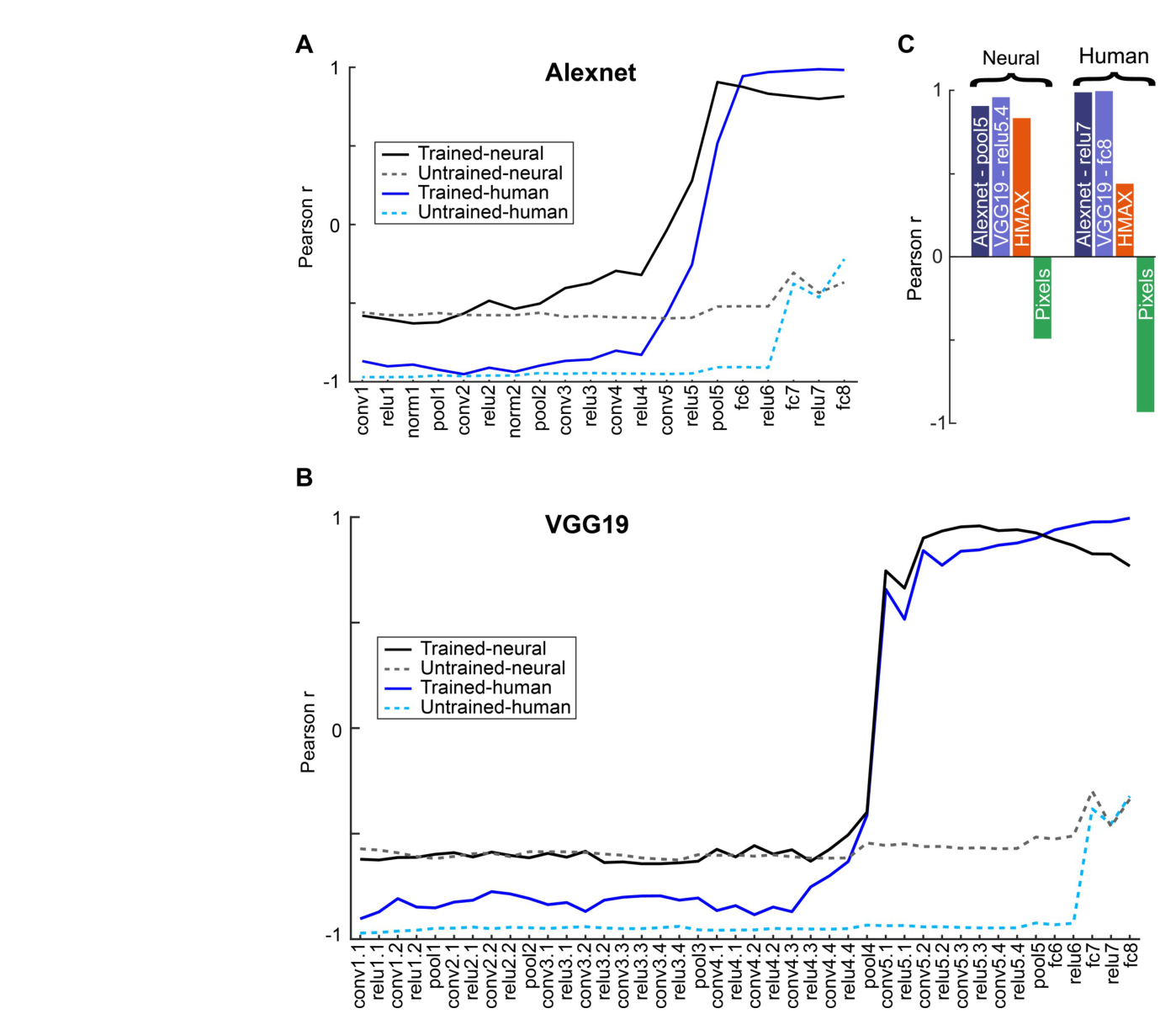
4. 在 Kayaert 的关键对比上，CNN 逐层复现了"IT → 人类"的模式切换。IT 对规则组内对、以及直/弯（ISC vs ISS）对比的反应调制大于三个不规则组内对，且直/弯对比的像素差其实更小（图 8A）；HMAX C2 复现不了这一模式（图 8C），人类判断则对直/弯对比相对规则形状更敏感（图 8B）。训练 VGG-19 的浅层距离贴合像素模式（与像素相关 0.966），到最深卷积层（conv5.4、pool5）已与 IT 模式几乎一致；而最后两层的距离模式转向人类判断——"ISC vs ISS 大于规则组距离"这一人类特征只在最深层显著（VGG-19 fc8 p=0.039；VGG-16 fc7 p=0.039、relu7/fc8 p=0.023；Alexnet 有趋势但未达显著）；所有未训练层都不像 IT 或人类（图 9、图 10）。就 6 组平均距离而言，IT 与最深卷积层的相关近乎完美，而人类判断与最后一个全连接层的相关趋近 1（图 10）；深层 CNN 对 IT 与人类数据的预测都优于 HMAX C2（图 10C）。

图注解读

图 1 · 64 个形状 stimulus 集：1 个规则组与 3 个不规则组

原文图注：Fig 1. Shape set. One group of Regular (R) and three groups of Irregular shapes: Irregular Complex (IC), Irregular Simple Curved (ISC) and Irregular Simple Straight (ISS). A group of 16 shapes corresponds to two consecutive rows (labeled a,b) and the group names are depicted in the tree graph on the right. The 8 pairs (a,b) of each group are defined by the numbers on top of the figure (1,2。 .8).

每两行为一组（a、b 行），共 4 组 64 个形状：R 组为规则几何形状（至少一个对称轴），组内 8 对的差异是 NAP（如边平行与否、轮廓直或弯）；ISC 为全曲线轮廓的不规则形状，ISS 由对应 ISC 把曲线换成直线而得（故同号列的 ISC 与 ISS 恰好差一个 NAP）；IC 则轮廓更多更复杂。各列跨组的 4 对在整体大小与长宽比上匹配、组间像素灰度差平衡。这张图是全部后续 RSA 的刺激字典，读懂组间结构才能理解"规则组内对 > 不规则组内对、直/弯对比大于组内对比"这些关键模式。

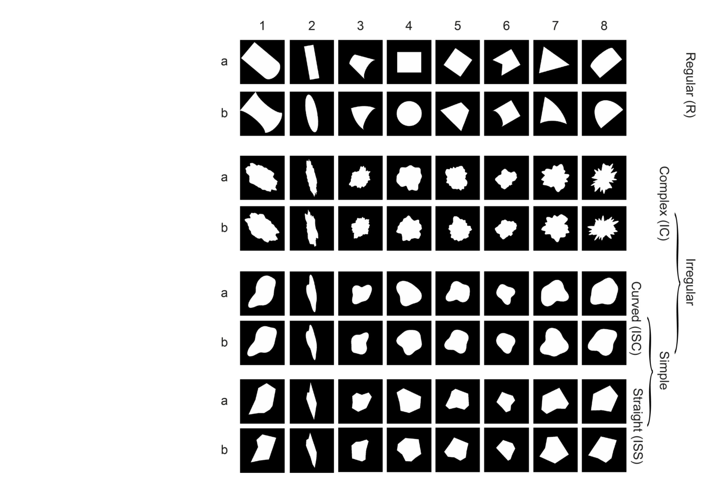
图 2 · 三个 CNN 的层级架构

原文图注：Fig 2. Model architectures. Deep Convolutional Neural Network (CNN) architectures for the 3 different networks that we employed: Alexnet, VGG-16 and VGG-19. Early computational blocks consist of consecutive operations such as: convolution (conv), RELU activation function, normalization (norm; only for Alexnet) and max pooling (pool). The later stages of each CNN incorporate three fully connected (fc) layers, where the first two are followed by a RELU activation function.

这是方法图的示意图：三个网络逐层列出，早期块由卷积、RELU、（仅 Alexnet 的）归一化与最大池化堆叠，末端为三个全连接层（前两个接 RELU）。读懂层名术语（conv1.1、pool5、relu7、fc8 等）是看图 3–7、9、10 横轴的前提；三个网络深度与单元数不同，正是检验"深度效应是否跨架构成立"的设计点。

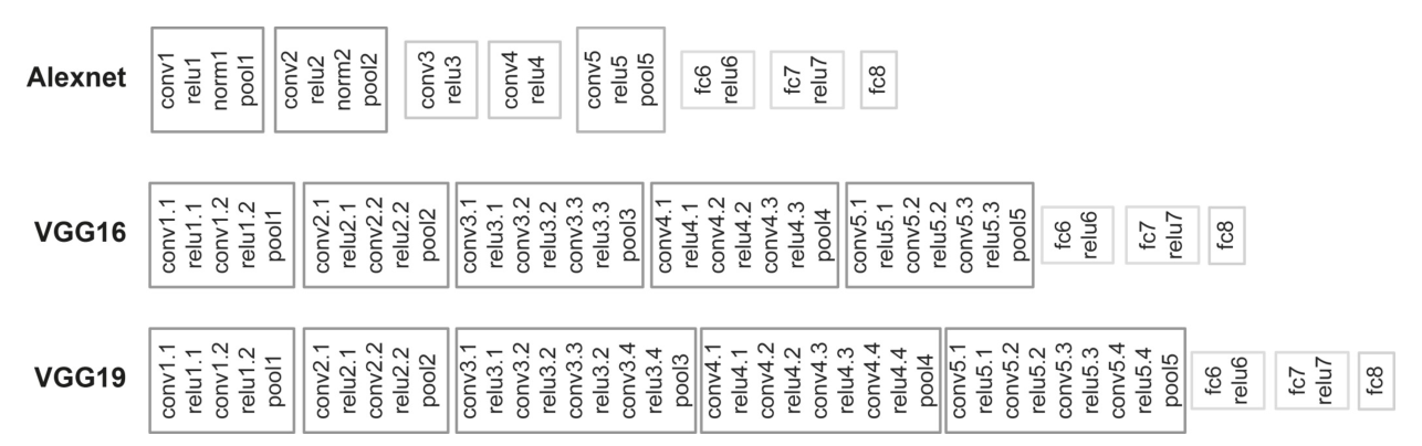
图 3 · 相异度矩阵：从像素到 IT 的逐层演变

原文图注：Fig 3. Dissimilarity matrices. Matrices of Euclidean distances for pixel gray-levels (A), the IT neurons (B), and 5 layers of the trained and untrained versions of 2 deep CNNs (C). Note that the dissimilarity matrices are by definition symmetric about the diagonal of zeros, which is plotted in white color. The stimulus groups are indicated in (A) as in Fig 1 and the CNN layers in (C) have the same terminology as in Fig 2. The matrices have been separately normalized and are plotted in percentile units. Dissimilarities increase from blue to yellow.

三个矩阵家族并排：像素灰度距离（A）、IT 神经元（B）、训练与未训练 CNN 各 5 层（C）；矩阵对称，对角线为零（白色），色标从蓝到黄表示相异度增大（各矩阵分别归一化为百分位单位）。读法是找块结构：IT 矩阵（B）里 R 组与 ISC/ISS 间呈现的特征块，在训练网络的深层矩阵中重现、在第一卷积层与未训练网络中缺席（后者更像像素矩阵 A）。这张图给出全篇结论 1、2 的直觉版：表征结构随训练逐层逼近 IT。

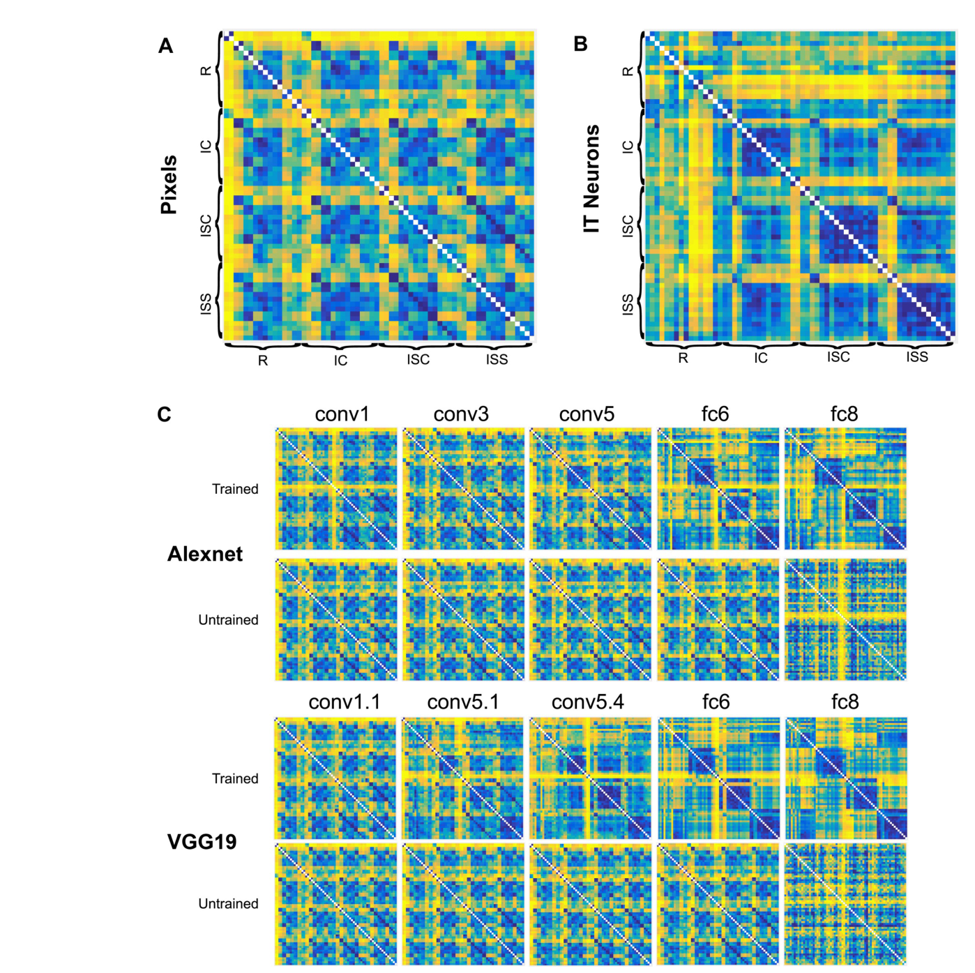
图 4 · IT–CNN 相关随层深的上升与全连接层的回落

原文图注：Fig 4. Representational similarity analysis of deep CNN layers and IT neurons for the whole shape set. Spearman rank correlation coefficients between IT and model layer similarities are shown for each layer of Alexnet (A) and VGG19 (B) using the Euclidean distance metric. Error bars depict 95% confidence intervals, determined by 10,000 bootstrap samples of the IT neuron pool (n = 119 neurons). Stars indicate layers for which the Spearman rank correlations for the trained version differed significantly from its untrained version (paired bootstrap test; False Discovery Rate corrected q<0.05). Crosses indicate trained layers which differed significantly from the first convolutional layer of the network. The horizontal line and gray band indicate the median and 95% interval, respectively, of the Spearman-Brown corrected split-half correlations (n = 10000 splits) of the neuronal distances, as an estimate of the noise ceiling.

横轴按架构排层、纵轴是 IT 与该层相异度的 Spearman 秩相关；实心点为训练版本，误差棒为 IT 池 10,000 次 bootstrap 的 95% 置信区间，星号=训练与未训练版本显著不同（FDR 校正 q<0.05），叉号=该训练层显著高于第一卷积层，水平灰带=对半相关估计的噪声天花板。读图：曲线随层深爬升、在最深卷积层达峰（ρ≈0.60）后在全连接层回落；星号集中出现在深层卷积层——这正是"训练效应=深度卷积层"的统计落点。支撑主要结果 1 与 2。

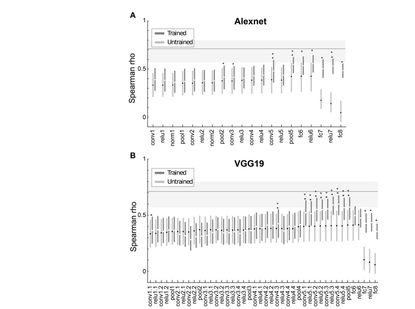
图 5 · 把形状缩小一半：相关跃升前移、峰值深度不变

原文图注：Fig 5. Representational similarity analysis of deep CNN layers and IT neurons for the whole shape set with two different sizes. Spearman rank correlation coefficients between IT and model layer similarities are shown for each layer of Alexnet (A) and VGG19 (B) for the original and twofold smaller sizes ("reduced size"). The dissimilarities were Euclidean distances. Error bars depict 95% confidence intervals, determined by 10,000 bootstrap samples of the IT neuron pool (n = 119 neurons). Stars indicate layers for which the Spearman rank correlations for the trained version differed significantly from its untrained version (paired bootstrap test; False Discovery Rate corrected q<0.05). The horizontal line and gray band indicate the median and 95% interval, respectively, of the Spearman-Brown corrected split-half correlations (n = 10000 splits) of the neuronal distances, as an estimate of the noise ceiling.

与图 4 同一画法，但每个网络画原始大小与缩小一半两条曲线。要点：小形状时 IT–CNN 相关在更浅的层就开始上升（感受野相对形状变大），但 VGG 的总体峰值仍出现在深层卷积层、两尺寸峰值高度接近；Alexnet 深层对小形状相关显著更高。此图回应"深度效应只是感受野问题吗"——大小有贡献，却不能解释峰值深度。支撑主要结果 2 的控制分析。

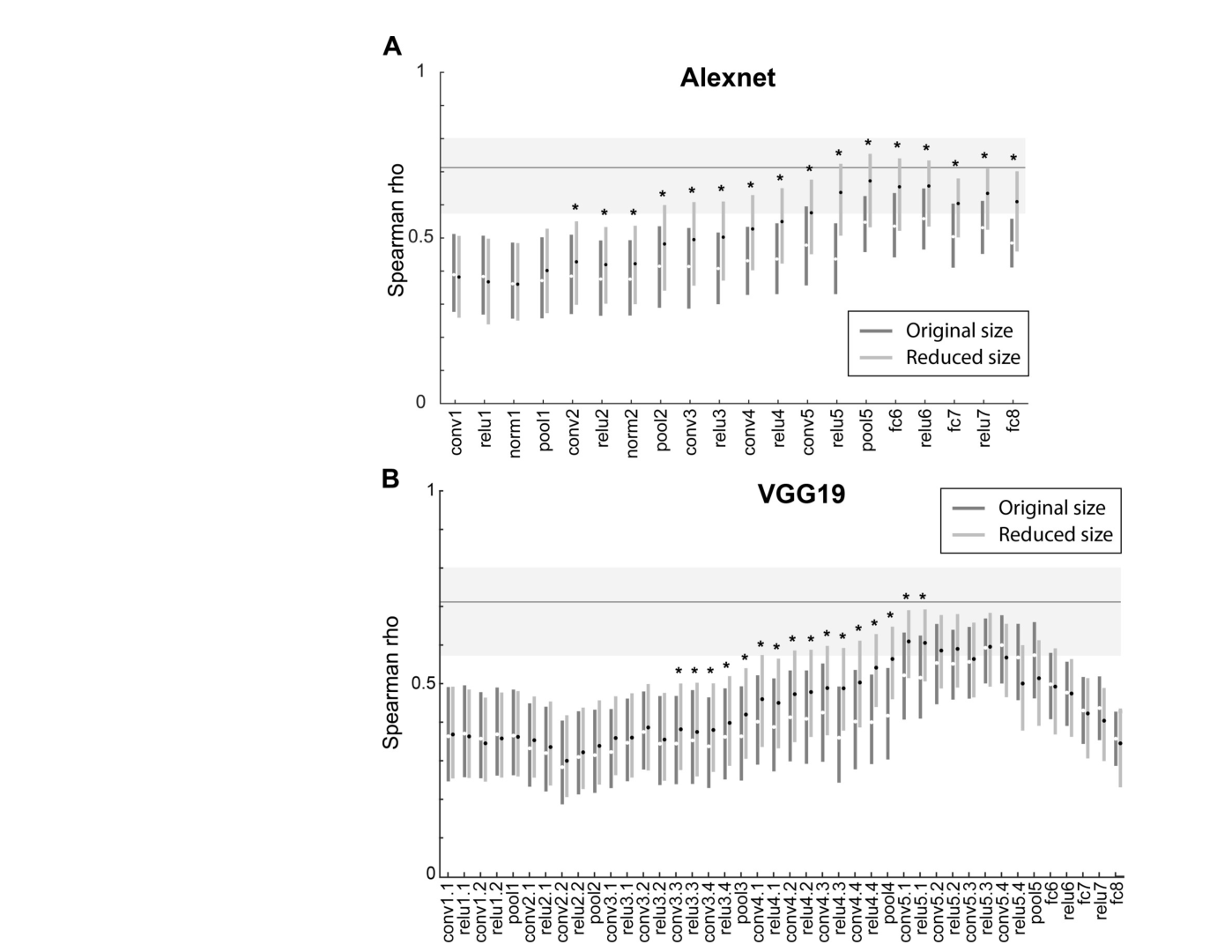
图 6 · 采样多少单元才够：表征高度冗余

原文图注：Fig 6. Similarities between IT and CNN peak layer shape dissimilarities as a function of percent of units. (A) Spearman rank correlation coefficients between IT and peak CNN layer similarities are shown for each of two CNN models as a function of sample size, expressed as percentage of the total number of units that were activated differentially by the 64 shapes. (B) Pearson correlation coefficients between the mean neural distances and the mean distances of the peak CNN layer (n = 6 mean distances; Fig 10) as a function of percentage of the total number of units. Note that 0.1% corresponds to only 3 Alexnet units, explaining the large range of correlations for that sample size. The dissimilarities were Euclidean distances. Error bars depict 95% confidence intervals, determined by 10,000 random samples from the population of differentially activated CNN units of that layer.

横轴是随机抽取的单元百分比，纵轴分别是全形状集的 IT–峰值层 Spearman 相关（A）和 6 组平均距离层面的 Pearson 相关（B），误差棒为 10,000 次抽样的 95% 区间。曲线在 10%（Alexnet）甚至 0.1%（VGG-19，约 100 个单元）处就已与全层重叠，且下界仍高于未训练网络水平——说明与 IT 的一致性分布在大量单元上，不是少数离群单元的功劳；0.1% 处 Alexnet 只剩 3 个单元，故区间极宽。支撑主要结果 3。

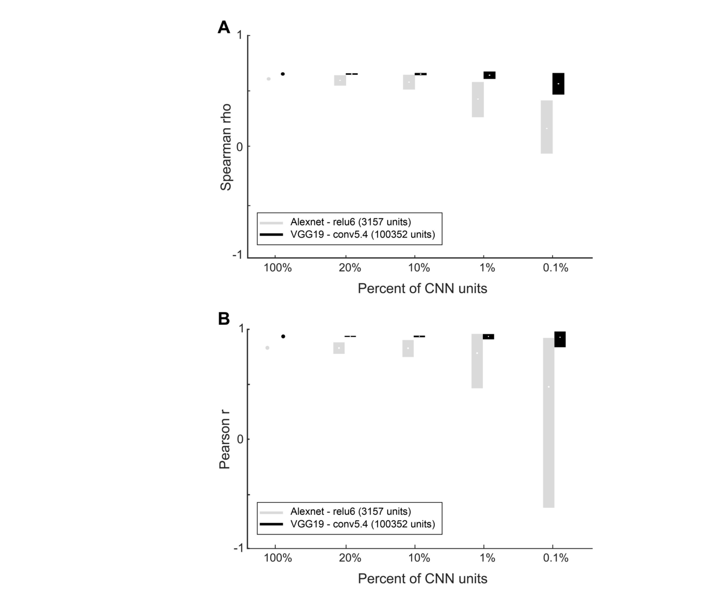
图 7 · 主成分维度：低维即可匹配 IT

原文图注：Fig 7. Similarities between IT and CNN peak layer shape dissimilarities as a function of retained principal components. (A) Spearman rank correlation coefficients between IT and peak CNN layer similarities are shown for each of two CNN models as a function of retained principal components of the CNN layer activations. The dissimilarities were Euclidean distances. Error bands depict 95% confidence intervals, determined by 10,000 bootstrap samples of the IT neuronal pool. (B) The cumulative proportion of explained variance as a function of principal component number for the Alexnet (black line) and VGG-19 layer (gray line). (C) Pearson correlation coefficients between the mean neural distances and the mean distances of the peak CNN layer as a function of retained principal components.

横轴为保留的主成分（PC）个数：(A) 全形状集 RSA 相关、(B) 累计解释方差、(C) 6 组平均距离相关。前 10 个 PC 已解释峰值层约 70% 方差；只留 3（Alexnet）或 5（VGG-19）个 PC，与 IT 的相关就达到用全层的水平（C 中需约 30 个 PC），说明 IT 相关的形状表征嵌在低维子空间、单元间高度冗余，但组水平模式的完美匹配需要相对高维的信息。支撑主要结果 3。

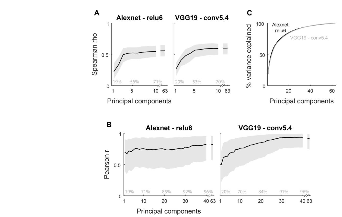
图 8 · 关键基线：IT、人类、HMAX 与像素的组间距离模式

原文图注：Fig 8. Response modulations for the shape groups: IT neurons, human judgements, HMAX and pixel-based dissimilarities. (A) Mean response modulations of IT neurons for the shape groups R, IC, ISC, ISS, "ISCa vs ISSa" and "ISCb vs ISSb". See Fig 1 for the nomenclature of the different shape groups. (B) Dissimilarities for the shape groups (R, IC, ISC, ISS, ISC vs ISS) based on human judgements. (C) Dissimilarities for the same shape groups based on the HMAX C2 layers' output. (D) Pixel-based dissimilarities. Error bars indicate standard errors of the mean. B, C and D are taken from Kayaert et al. [12].

四幅柱状图对比同一批组间比较（R、IC、ISC、ISS 组内对与"ISCa vs ISSa"/"ISCb vs ISSb"跨组对）的平均距离：(A) IT——规则组内对大于三个不规则组内对，直/弯对大于一切组内对，尽管其像素差最小；(B) 人类——直/弯对比规则形状的相对敏感度高于 IT；(C) HMAX C2——没有呈现 IT 的那种直/弯优势模式；(D) 像素——与 IT 模式近乎反向（这是设计使然：NAP 差异的像素差被刻意做小）。误差棒为均值标准误。这张图是"生物基线"，图 9、10 都拿它当参照。支撑主要结果 4 的前半。

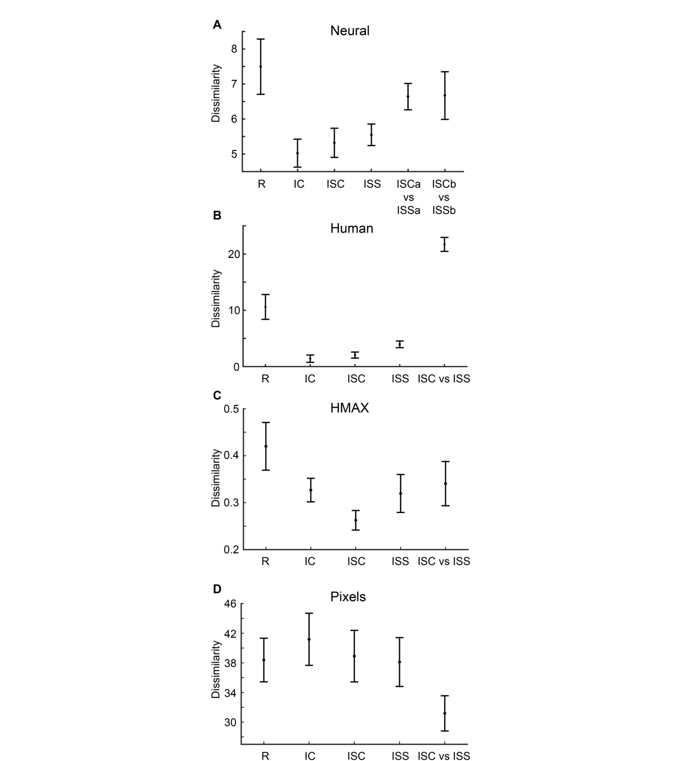
图 9 · CNN 逐层的组间距离：浅层像素相、深层 IT 相、末层人类相

原文图注：Fig 9. Response dissimilarities for the shape groups: Deep CNN layers. Dissimilarities for groups R, IC, ISC, ISS, "ISCa vs ISSa", "ISCb vs ISSb" of selected trained (left column) and untrained (right column) versions of VGG-19 layers (same nomenclature as in Fig 2). Same conventions as in Fig 8. The specific selection of layers is motivated by the fact that there were no critical differences in the layers that follow the selected ones.

左列为训练版 VGG-19 的选定层，右列为未训练版，各层沿用图 8 的柱状与坐标约定。逐层往下读：conv1.1 的模式几乎就是图 8D 的像素模式；到 conv5.4/pool5 模式变得与图 8A 的 IT 模式高度相似；relu7、fc8 则转向图 8B 的人类模式（直/弯对高于规则对）。右列各层都更像像素模式，没有一层复现 IT 或人类。这张图把"三层相"的叙事（像素→IT→人类）可视化，是全文结论最直观的一张图。支撑主要结果 4。

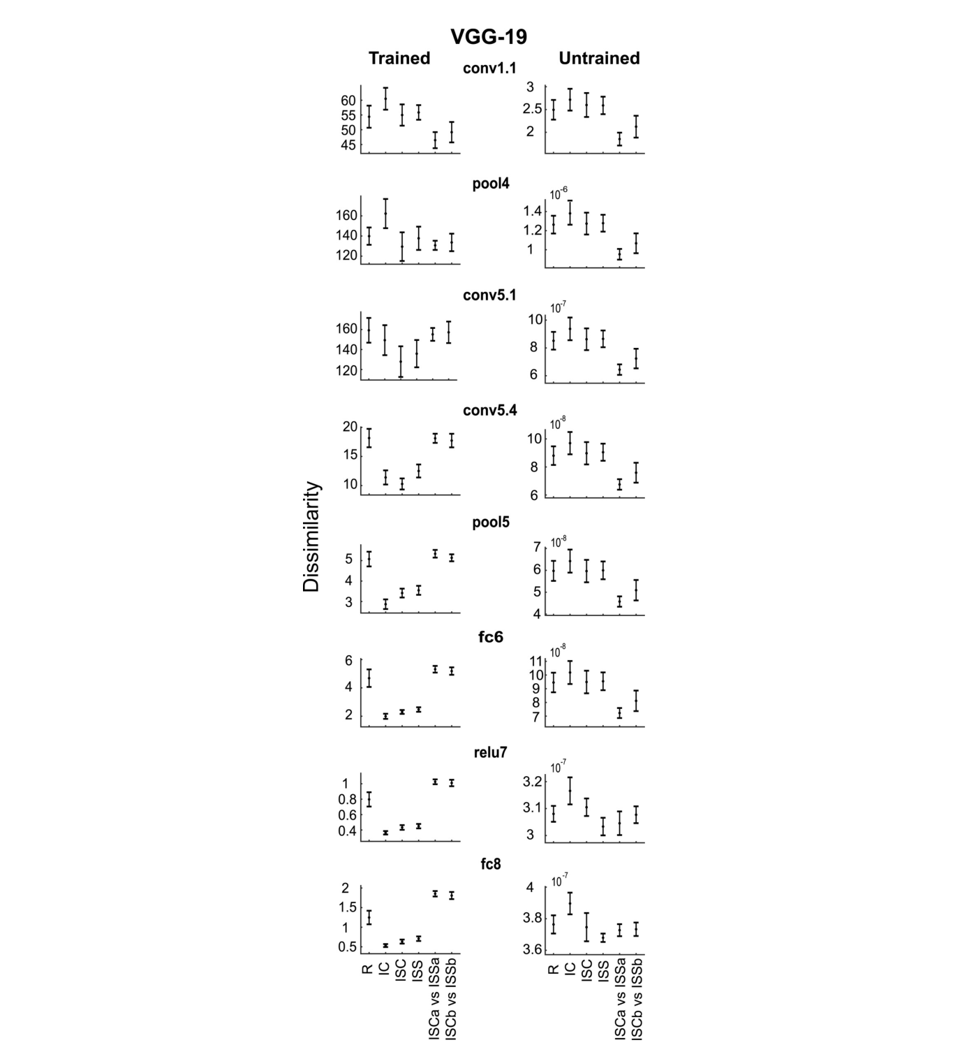
图 10 · 与生物数据的逐层相关曲线及 HMAX 对照

原文图注：Fig 10. Correspondence between model dissimilarities and biological dissimilarities (IT responses and human judgement-based dissimilarities) for the shape groups. (A, B). Gray curves show the Pearson correlation coefficients between the mean neural distances and the mean distances of the CNN layers (n = 6 mean distances per layer). Blue curves show the Pearson correlation coefficients of the CNN layer distances and the distances based on human judgements. Data for trained and untrained CNNs are plotted with full and dashed lines, respectively. Nomenclature of CNN layers as in Fig 2. Results for all two models (Alexnet and VGG-19) are displayed in the subplots (A, B). (C) Neural: Pearson correlation coefficient between the mean IT distances and the mean distances of the peak Alexnet layer, peak VGG-19 layer, the mean HMAX C2 layer distances, and mean pixel-based distances, across shape groups. Human: same for the human judgement distances.

(A)(B) 横轴为层、纵轴为 Pearson 相关：灰线=该层与 IT 六组平均距离的相关，蓝线=与人类判断距离的相关，实线=训练版、虚线=未训练版。(C) 汇总柱状：峰值层、HMAX C2、像素距离分别对 IT 与人类数据的相关。读图：灰线在浅层为负（因像素差与神经差近乎反向，系刺激设计所致），在训练版深层卷积处陡升、到全连接层回落；蓝线则沿训练版全连接层持续上升、末层趋近 1。(C) 显示深层 CNN 对两种生物数据的拟合都好于 HMAX C2 与像素。支撑主要结果 1、4 的量化总结。

讨论

作者的解读分三层。其一，这是对 CNN 作为 IT 模型的一次强泛化检验：参数完全由"分类自然图像"这一目标决定、从未见过这些剪影形状，深层卷积层却复现了 IT 的抽象形状相似结构——模型解释力并非只对自然图像家族成立。其二，为何最深全连接层反而偏离 IT？作者解释为该层已处于分类决策端、被训练标签强驱动，而 IT 神经元对同一语义类别的不同范例缺乏不变性（与 Vogels 1999、Popivanov 2014 的观察一致，也与最深 CNN 单元的类内不变性相反）；人类排序对直/弯的额外敏感与末层一致，可能因为排序任务本身会被高阶分类策略"侵入"。其三，方法学倡议：作者特别强调未训练 CNN 作为对照的价值——它把架构属性（浅层局部感受野平铺、非线性池化）与训练效应拆开，并建议未来研究都把未训练网络当基准。局限方面，作者承认形状性质并未穷尽（结论未必外推到未操纵的维度）、CNN 对噪声/遮挡/对抗样本比人类脆弱、层与脑区的对应（皮层层内 laminae、时间加工阶段）基本未解，且生物系统在个体发育中塑造形状选择性的学习算法未必是监督式的。与 Kubilius 等人的 NAP 优势研究、Kayaert 原始研究及 Kriegeskorte 的 RSA 框架直接对话。

一句话总结

这篇论文我最欣赏的是那个"三层相"的发现：同一个训练好的 CNN，中层像猴 IT、末层像人判断，说明"感知相似性"与"被类别标签重塑的判断"在网络里是两个相邻但可分离的阶段。以我的理解，未训练对照的引入是全文方法论上最干净的一步——它把"像 IT"从架构的偶然变成训练的成就；当然 119 个神经元池与 64 个抽象形状的泛化边界，作者自己也标注得很诚实。