本研究阐明了灵长类大脑下颞叶面孔处理网络编码个体面孔身份的计算原理:将任意人脸参数化映射为 50 维“面孔空间”(face space)中的一个坐标向量,单个面孔选择性神经元的动作电位发放率正比于该面孔向量在其偏好轴上的线性投影。基于约 200 个面孔神经元的群体放电模式即可线性重构出受试猕猴所观察到的面孔图像,同时基于该线性轴投影模型亦能预测单个神经元的发放反应。研究通过设计在调谐正交平面内具有相同投影的“感元面孔”(metamers),证实了先前被假定为特异性表征个体身份的稀疏前内侧 patch(AM)神经元同样遵循线性轴投影机制,为理解高级视皮层的特征表征提供了显式计算模型。
研究背景
揭示大脑如何表征高维复杂物体的个体身份是视觉神经科学的核心问题之一。灵长类腹侧视流通路末端的下颞叶(IT)皮层在维持复杂物体身份表征的同时,对视网膜成像的几何变换(如尺寸缩放、位置平移与视角偏转)表现出知觉容忍性(Ito 等 1995;Brincat & Connor 2004;Majaj 等 2015)。然而,单个 IT 神经元遵循何种计算编码规则长期存在争议:多数 IT 神经元对多类复杂图形呈现宽泛的放电响应,难以用解析模型完全拟合。由于自视网膜至 IT 皮层经历了多级非线性前馈计算,早先研究推测高级视皮层单神经元反应可能难以通过简化的显式线性模型予以完整刻画(Yamins 等 2014 的层级卷积网络对 IT 神经元放电方差的解释率不足一半)。
作者选择面孔识别系统作为突破口:其一,功能磁共振成像(fMRI)证实猕猴大脑颞下叶存在一系列相互连接、高度特化的面孔加工功能区(face patches),其内部神经元呈现出极高的面孔选择性(Tsao 等 2006);其中前内侧 patch(AM)包含对特定面孔具有高度稀疏选择性且具备跨视角不变性的神经元(Freiwald & Tsao 2010),常被类比为表征具体个体的“样例细胞”(exemplar-based coding;Quiroga 等 2005);其二,面孔刺激具有高度规范的几何构型,能够利用统计形貌模型投影至由连续特征参数界定的“面孔空间”,为遍历神经元调谐几何特性提供了实验条件。现有研究需要明确:IT 面孔神经元究竟是在执行以某特定样例为中心的高维径向距离度量(样例模型,Riesenhuber & Poggio 1999;Valentine 1991),还是对高维特征轴进行线性投影度量(轴模型)。
研究思路
研究采取“参数化空间构建 → 神经调控几何测绘 → 双向编解码实验验证”的技术路线:第一步,基于主动外观模型(AAM,Cootes 等 2001)将 200 张真实人类面孔图像库进行参数化分解:在每张面孔上标注 58 个关键特征点,特征点二维坐标提取为面孔形状(shape)特征;通过将特征点平滑变形对齐至平均基准网格,剥离空间形变后得到表征纹理色调的无形形状外观(shape-free appearance)特征;分别对形状与外观矩阵实施主成分分析(PCA),各自截取前 25 个主成分,构建出正交的 50 维面孔空间——空间中任意坐标点均可通过逆变换合成一张写实的人脸图像,确保特征维度的生态有效性;第二步,在 50 维空间中随机均匀采样生成 2000 张面孔刺激,在体记录面孔 patch 神经元放电,利用尖峰触发平均(STA)提取各个神经元在 50 维特征空间中的最优调谐轴,以检验“轴模型”(放电率取决于面孔向量在 STA 轴上的投影值)与“样例模型”(放电率取决于到模板面孔的欧氏距离)的契合度。
轴模型具有可证伪的理论推论:神经元在与 STA 正交的“零子空间”(null space)内,对特征值发生改变的面孔应当维持恒定放电。作者为此设计了三重检验:计算垂直于 STA 轴的正交调谐曲线形态、在线定向合成位于零子空间内的感元面孔测试神经反应,以及评估两类模型对独立测试集神经放电率的泛化预测能力。
方法
实验受试为两只成年雄性恒河猴(7–9 岁)。采用 3T fMRI(配合超顺磁氧化铁造影剂 Feraheme,对比面孔与人造物体的 BOLD 激活)定位全脑面孔功能区,将慢性微电极记录位点精准引导至中侧/中沟底 patch(ML/MF)以及前内侧 patch(AM)。使用高阻抗钨丝微电极记录单单元动作电位;通过 16 张面孔与 80 张非面孔物体的快速筛选,选取面孔选择性指数 FSI > 0.33 的神经元进入主实验,两只猴合计记录到 205 个单单元(猴 1:ML/MF 51 个、AM 64 个;猴 2:ML/MF 55 个、AM 35 个)。在注视任务中,面孔刺激中央视场呈现(视视角 5.7°),每张图片呈现 150 ms,间隔 150 ms 灰屏,每张刺激重复 3–5 次,以红外眼动仪监控注视位置;放电计数时间窗设定为刺激呈现后 50–300 ms。
数据分析方法:将 50 维刺激向量以神经元放电脉冲数为权重求均值,计算尖峰触发平均(STA)向量;通过外观维与形状维 STA 向量长度之比定义“形状偏好指数”(SP);沿 STA 轴将刺激特征值划分为 16 等分计算调谐响应曲线,利用移位预测器检验统计显著性;解码端采用留一交叉验证的多元线性回归,基于群体神经反应预测未知面孔的 50 维特征向量,并通过欧氏距离最近邻算法评估整体面孔识别准确率;组织 78 名人类受试者在线开展二选一迫选心理物理学测验以评估重建面孔的保真度。模型拟合评估采用三阶多项式非线性拟合与梯度下降算法,样例模型、最大池化视角不变模型、深层卷积神经网络特征单元以及传统特征脸(Eigenface)模型均在相同神经稀疏度与噪声约束下进行基准对齐。
主要结果
-
中位面孔 patch(ML/MF)与前位 patch(AM)呈现互补的特征调谐分离。记录神经元平均显著调谐于 6.1 个特征维度(范围 0–17)。形状偏好指数分析显示,ML/MF 神经元多数对形状特征维度的调谐显著强于外观维度,而 AM 神经元则表现出相反的偏好,主要调谐于无形形状外观维度(图 1E–H,群体均值差异 p=10⁻²⁵)。这一解剖分工与既往电生理一致:ML/MF 主要表征特定视角的局部几何,AM 负责表征跨视角的个体身份(Freiwald & Tsao 2010)。所有神经元沿各自的 STA 轴均呈现单调上升的“斜坡式”(ramp-like)调谐,极值特征值诱发最高或最低放电(图 1I–K)。
-
线性解码算法可从群体放电中稳定重构任意输入面孔。对 2000 张面孔特征采用留一交叉验证线性回归,单维特征预测与真实值吻合良好(图 2B);外观维度在 AM 神经元中解码精度更高,形状维度在 ML/MF 神经元中解码表现更好(图 2C)。利用 205 个神经元合并的群体放电模式预测全部 50 维特征后,可逆向合成三维人脸图像:仅依赖 AM 群体即可重构出高度保真的面孔,融合 ML/MF 数据后重构质量进一步提升(图 3A)。在 40 张干扰面孔候选集二选一测试中,合并群体的解码识别率达到 75%,显著高于随机基线(图 3B);在控制神经元采样数量时,融合群体相比单一脑区展现出更快的解码性能增长(n=99 时,合并 vs AM p<0.01、vs ML/MF p<0.005;图 3C)。人类受试者在二选一迫选测试中识别重构面孔的准确率达 88.3%(p=6×10⁻⁶²),在 40 选一测试中识别率依然达到 69.6%(p=6×10⁻²⁴)。
-
神经元在正交子空间内的调谐曲线趋于平坦,符合线性轴编码特征。AM 神经元(包含表现出高稀疏发放特性的单元)沿垂直于 STA 轴的各个正交方向的平均调谐曲线保持平直,未见高斯钟形调谐特征(图 4A);相比之下,基于模板距离匹配的样例模型与最大池化视角模型在相同约束下均表现出显著的钟形径向调谐(图 4B),在各神经稀疏度区间内 AM 神经元的正交非线性显著低于样例模型(图 4F,各组 p<0.001)。这一正交平坦特性证实神经元放电取决于特征向量的一维线性投影,而非高维距离,解释了为何极度稀疏的 AM 神经元可能对若干在几何形态上截然不同的面孔产生相似放电——这些面孔在神经元的零子空间中落于相同的投影标量上(图 4D)。ML/MF 神经元在形状特征空间中同样表现出一致的轴编码规律(补充图 S4M、N)。
-
轴模型预测神经放电率的表现接近生理测量噪声天花板。利用 1900 张面孔训练、100 张重复刺激测试,轴模型对 AM 神经元放电方差的平均解释率达到 56.9%(峰值达 68%),显著高于样例模型的 41.7%(配对 t 检验 p<0.001;图 4H、I);经 Spearman-Brown 校正后,实验测量的理论可解释方差天花板为 71.1%,轴模型达到了该噪声上限的 80.0%,明显优于卷积神经网络单元的 48.5%。任务训练卷积网络的输出单元仅能解释 30% 方差(图 4K),基于像素 PCA 的 Eigenface 模型解释率为 31%(图 4L)。通过在线定向合成落在“STA 轴 × 主正交轴”二维平面内的 144 张感元面孔并回录测试,22 个 AM 神经元在正交轴上的调谐方差仅为 STA 轴调谐方差的 8.5%(单样本 t 检验 p=2×10⁻³⁴),在受控干预实验中验证了轴模型的预测(图 5)。
-
轴编码机制支持跨视角知觉容忍性并在计算效率上具备理论优势。采用 2000 张正面与共轭参数化侧面面孔开展记录(46 个 AM 细胞):同一神经元的正面与侧面 STA 向量在外观维度上呈现高度跨视角相关(图 6B–D),且外观偏好越强的神经元跨视角相关系数越高(图 6F);利用 46 个神经元的固定线性模型能够跨视角解码并重构侧面面孔图像(图 6G–I)。神经网络仿真表明:在高维特征空间(维度 >6)中,基于轴投影的分类能力与基于欧氏距离的分类表现相当;然而轴度量网络具备更高的表征紧凑度(在输入单元受限时显著占优),且具有更优的抗噪声干扰能力(图 7)。
图注解读
图 1 · AM 与 ML/MF 群体对面孔特征的互补表征
原文图注:Figure 1. Complementary Representation of Facial Features by AM and ML/MF Populations (A–C) Generation of parameterized face stimuli. (A) 58 landmark points were labeled on 200 facial images from a face database (FEI face database; example image shown on left). The positions of these landmarks carry shape information about each facial image (middle). The landmarks were smoothly morphed to match the average landmark positions in the 200 faces, generating an image carrying shape-free appearance information about each face (right). (B) PCA was performed to extract the feature dimensions that account for the largest variability in the database. The first principal component for shape (B1) and appearance (B2) are shown. (C) Example face stimuli generated by randomly drawing from a face space constructed by the first 25 shape PCs and first 25 appearance PCs. (D) Spike-triggered average of a face-selective neuron from anterior face patch AM. (E) Vector length of the STA for the 25 appearance dimensions is plotted against that for the 25 shape dimensions for all the cells recorded from middle face patches ML/MF (blue) and anterior face patch AM (red). (F) Distribution of shape preference indices... (G) Reliability of the estimated population average of shape preference index for ML/MF and AM... (H) Number of significantly tuned cells (p < 0.01 by shift predictor) for each of 50 dimensions for ML/MF and AM cells in both monkeys. (I) Response of a neuron in AM is plotted against distance between the stimulus and the average face along the STA axis. (J) Responses of ML/MF (left) and AM (right) neurons as a function of the distance along STA dimension. (K) Neuronal responses as a function of the feature value for the first shape dimension (top) and first appearance dimension (bottom) for all significant cells.
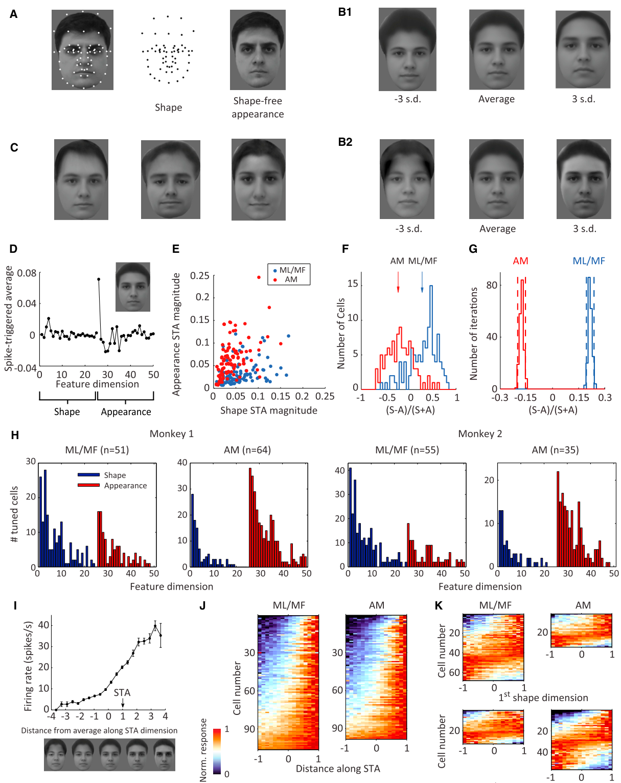
读图说明:(A–C) 呈现参数化面孔空间的生成流程:标定 58 个关键解剖位点提取形状,对齐至平均基准提取无形外观,经 PCA 各取前 25 个主成分组合为 50 维空间,(C) 展示空间中的随机采样样本;(D) 展示 AM 单个面孔神经元的 STA 向量及对应的特征面孔;(E–H) 揭示解剖功能分离:散点图 (E) 与分布图 (F) 证实 ML/MF 群体(蓝色)显著偏向形状维度调谐,AM 群体(红色)显著偏向外观维度调谐(p=10⁻²⁵),(H) 给出各维度显著调谐细胞数量分布;(I–K) 描绘单细胞放电随 STA 轴特征距离的变化,呈现单调上升的斜坡式曲线。该图确立了特征空间架构及解剖亚区的功能分工,支撑主要结果第 1 条。
图 2 · 用线性回归解码面孔特征
原文图注:Figure 2. Decoding Facial Features Using Linear Regression (A) Diagram illustrating decoding model. To construct and test the model, we used responses of AM (n = 99) and ML/MF (n = 106) cells to 2,000 faces. Population responses to 1,999 faces were used to determine the transformation from responses to feature values by linear regression, and then the feature values of the remaining image were predicted. (B) Model predictions using AM data are plotted against actual feature values for the first appearance dimension (26th dimension). (C) Percentage explained variances for all 50 dimensions using linear regression based on responses of three different neuronal populations: 106 ML/MF cells (blue); 99 AM cells (red); 205 cells combined (black). (D) Decoding accuracy as a function of the number of faces randomly drawn from the stimulus set for three different models.
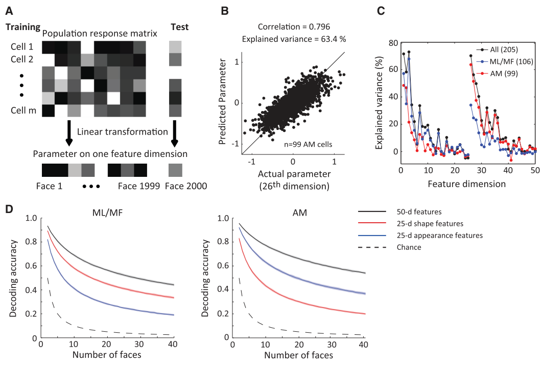
读图说明:(A) 描绘多元线性回归留一交叉验证解码流程;(B) 展示利用 AM 放电模式预测第一外观主成分特征值与真实值的散点分布,数据点贴近恒等线;(C) 绘制 50 个特征维度上的解码可解释方差,外观维度(右侧)在 AM 群体中表现更优,形状维度(左侧)在 ML/MF 中表现更优,合并群体在各维度均达最佳;(D) 绘制分类解码正确率随干扰面孔数量增加的变化曲线,合并群体识别表现优于单一脑区。该图支撑主要结果第 2 条。
图 3 · 从神经反应重建面孔图像
原文图注:Figure 3. Reconstruction of Facial Images Using Linear Regression (A) Using facial features decoded by linear regression in Figure 2, facial images could be reconstructed. Predicted faces by three neuronal populations and the corresponding actual stimuli presented in the experiment are shown. (B) Decoding accuracy as function of number of faces, using a Euclidean distance model (black solid line). Decoding accuracy based on two alternative models, nearest neighbor in the space of population response (gray dashed line, see STAR Methods) and average of nearest 50 neighbors (gray solid line), were much lower. The black dashed line represents chance level. In the left panel, boxes and error bars represent mean and SEM of subjective (human-based) decoding accuracy based on 78 human participants. (C) Decoding accuracy for 40 faces plotted against different numbers of cells randomly drawn from three populations (black, all; blue, ML/MF; red, AM).
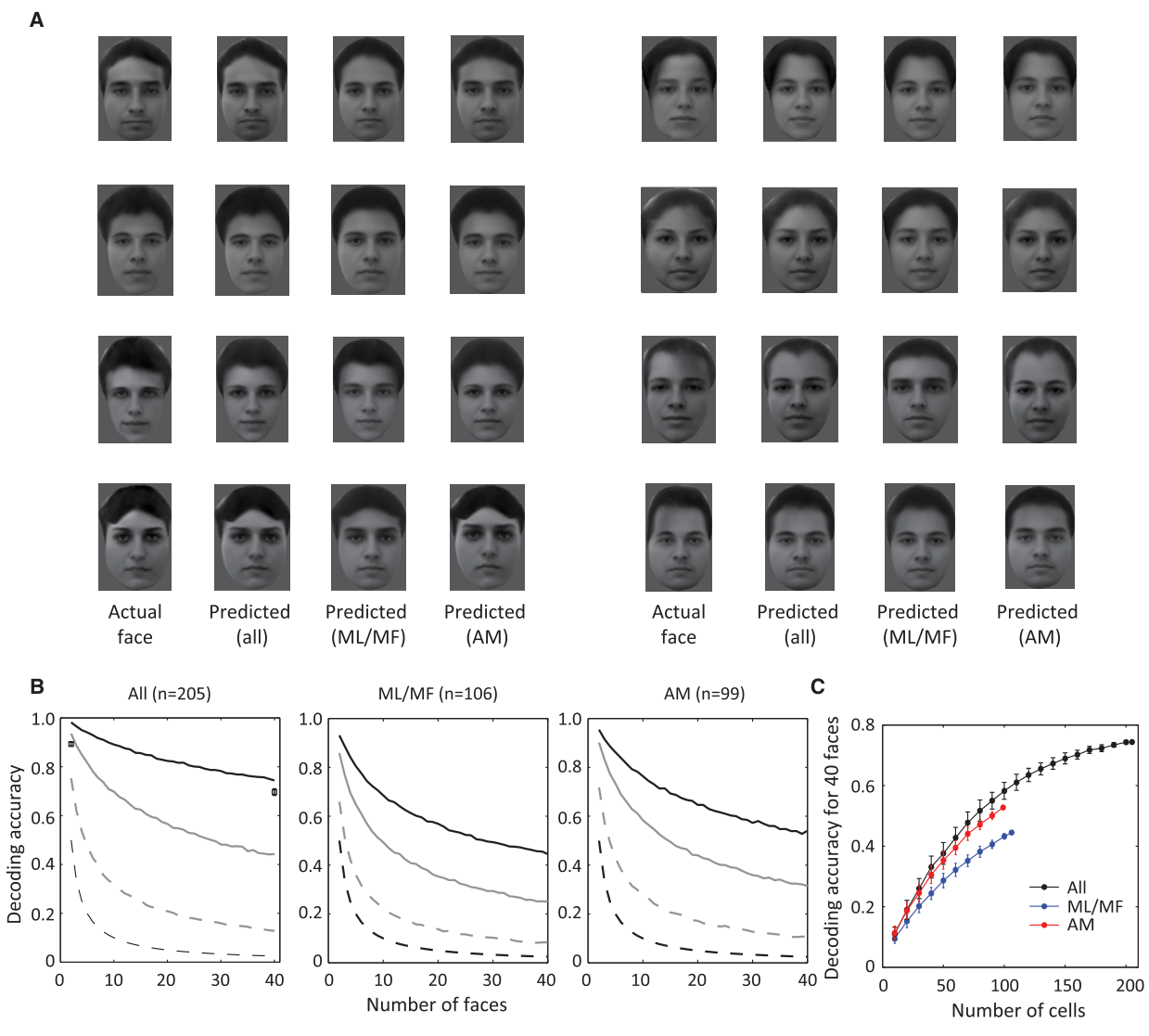
读图说明:(A) 呈现实际测试面孔与分别依据 ML/MF、AM 及合并群体放电重构的人脸图像对比,展现图像视觉保真度;(B) 比较基于解码特征欧氏距离与基于原始放电向量最近邻的客观识别率,证实先线性提取空间坐标再比对距离的模型表现更优,左侧嵌图为 78 名人类受试者的主观识别正确率;(C) 在控制抽取神经元数量时评估识别准确率,合并群体曲线高于单一脑区子集。该图支撑主要结果第 2 条。
图 4 · AM 细胞在 STA 正交轴上近乎平坦的调谐
原文图注:Figure 4. AM Neurons Display Almost Flat Tuning along Axes Orthogonal to the STA in Face Space (A) For each neuron in AM, the STA was first computed, and then 2,000 random axes were selected and orthogonalized to the STA in the 25-d space of appearance features. Tuning functions along 300 axes accounting for the largest variability in the stimuli were averaged and fitted with a Gaussian function. (B) Same as (A), but for two control models. (B1) Each simulated cell corresponds to one of the 200 real faces projected onto the 25-d face space of appearance features (exemplar face)... (B2) Each simulated cell corresponds to 81 transforms of a single identity (nine views*nine positions)... (C) Responses of an AM neuron to 25 parameterized faces... (D) Responses of the cell in (C) to different faces are color coded and plotted in the 2-D space spanned by the STA axis and the axis orthogonal to STA... (E) Same as (D), but for a non-sparse AM cell. (F) ...The difference between AM neurons and two models was significant for all three sparseness levels (p < 0.001, Student's t test). (G–L) Two models were used to fit face cells' responses to parameterized face stimuli: (1) an "axis" model... (2) an "exemplar" model... (H) Predicted versus actual responses for one example cell using an axis model. The model explained 68% of variance. (I) ...An axis model provides significantly better fits to actual responses (mean = 56.9%) than an exemplar model (mean = 41.7%, p < 0.001, paired t test). (J) ...Percentage variances explained, after Spearman-Brown correction (mean = 71.1%)... (K) A convolutional neural net was trained to perform view-invariant face identification... (L) Neuronal responses were fitted by a different "axis" model using "Eigenface" features...
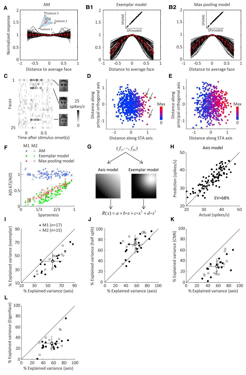
读图说明:(A) 绘制 AM 神经元在正交于 STA 轴的 300 个方差最大维度上的平均调谐曲线,数据点呈现水平直线分布;(B) 样例模型与多视角池化模型在相同正交轴上均表现出典型的钟形衰减;(C–E) 稀疏 AM 神经元单细胞放电热图,在 STA × 正交轴平面上放电率仅随 STA 轴变化,证实零空间内不同外观面孔具有等价响应;(F) 各稀疏度分级下 AM 神经元正交非线性均显著低于模型;(G–L) 模型定量拟合分析:轴模型预测方差(均值 56.9%)显著优于样例模型(41.7%,p<0.001),达到理论噪声天花板(71.1%)的 80.0%,并优于 CNN 单元与特征脸基底。该图支撑主要结果第 3、4 条。
图 5 · 为每个细胞定向合成的感元脸
原文图注:Figure 5. Responses of AM Cells to Faces Specifically Engineered for Each Cell Confirms the Axis Model (A) Experimental procedure. After recording the responses of a face cell to 2,000 parameterized face stimuli, the STA axis and the principal orthogonal axis were extracted. Facial features were evenly sampled along each axis, and a facial image was synthesized for each pair of features. The synthesized images were presented to the monkey, and responses of the same face cell were recorded. (B) The responses of an AM cell to 144 faces evenly sampled from the 2-d space spanned by the STA axis and principal orthogonal axis, synthesized specifically for this cell, are color coded and plotted. (C) The responses of the cell in (B) are plotted against the distance along the STA axis and two orthogonal axes. (D) Responses of four more example cells are color coded and plotted. (E) (E1) Responses of 22 cells are plotted against the corresponding STA axes (red) and principal orthogonal axes (black). (E2) The SDs of the projected responses along the orthogonal axes are compared to the STA axes... On average, the tuning along the orthogonal axes is 8.5% of the tuning along the STA axis, and significantly smaller than 1 (one-sample t test, p = 2*10-34).
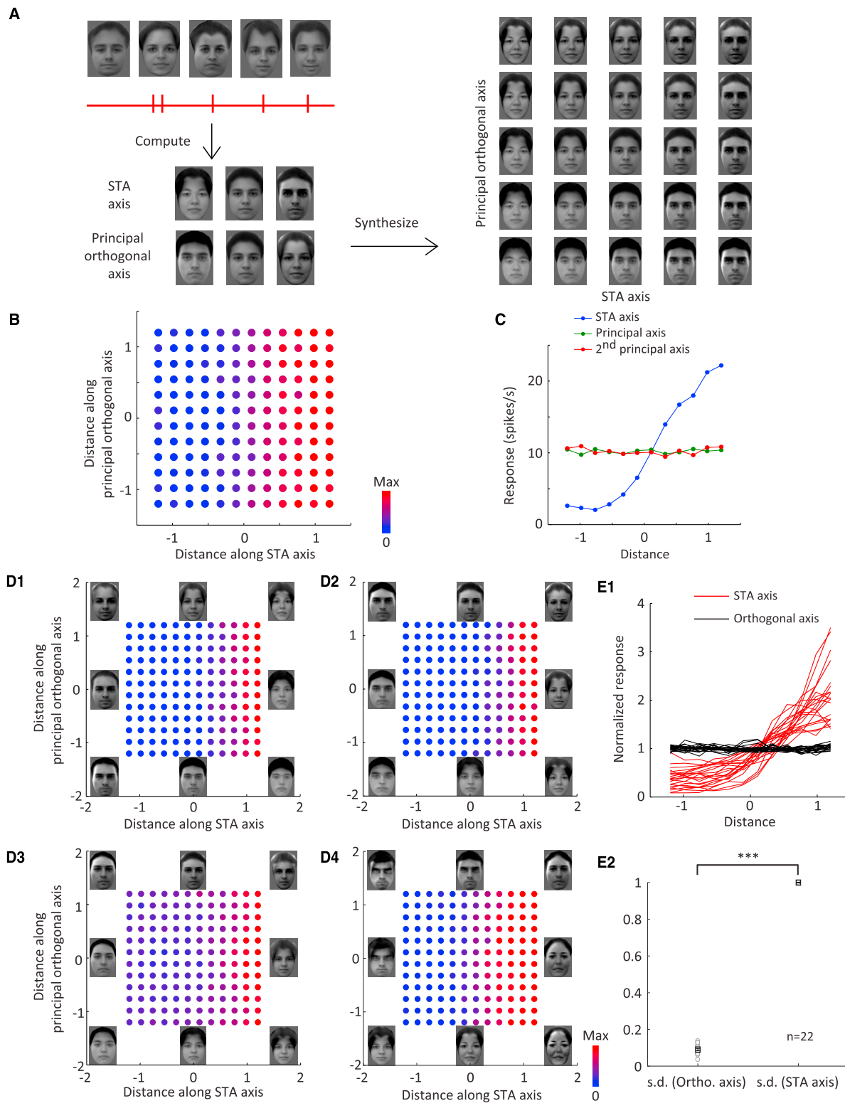
读图说明:(A) 呈现闭环合成验证协议:在体提取 STA 轴与主正交轴后,在线采样合成 144 张二维平面网格面孔回放测试;(B) 单细胞在 144 张感元面孔刺激下的放电率热图,放电强度仅随横轴(STA 轴)单调改变,垂直正交轴无调节效应;(C) 沿不同轴向的放电响应曲线;(D) 另外 4 个代表性细胞的放电热图;(E) 22 个 AM 神经元汇总分析表明,正交轴调谐方差平均仅为 STA 轴的 8.5%(p=2×10⁻³⁴)。该因果性实验直接验证了主要结果第 4 条中的轴模型假说。
图 6 · 轴编码模型对视角变化容忍
原文图注:Figure 6. The Axis Coding Model Is View Tolerant (A) To explore how our model could be extended to other views besides frontal, parameterized faces of right profiles were generated whose main dimensions were conjugate to those of the 2,000 frontal faces (see STAR Methods). The first PCs for shape features and appearance features of the profile face space are shown. (B) Spike-triggered average computed using 2,000 frontal stimuli (black) and 2,000 profile stimuli (red) for an example cell in AM. (C) Correlation between profile STA and frontal STA on one single feature dimension (first appearance dimension) across n = 46 AM neurons. Solid and open circles indicate data from two different monkeys. (D) STA correlation across cells for all 50 dimensions. Shaded regions indicate 99% confidence intervals of randomly shuffled data. (E) Response of the neuron in (B) is plotted against distances between the stimuli and the average face along the STA axis for frontal and profile stimuli. (F) The relationship between face view invariance and feature preference for frontal images across cells. (G–I) For the set of 4,000 faces, including 2,000 frontal and 2,000 profile faces, we trained a linear model to predict features on individual dimensions based on population responses of 46 AM cells... (H) Four reconstructions of profile faces... (I) Decoding accuracy as a function of the number of faces... shown separately for frontal and profile faces.
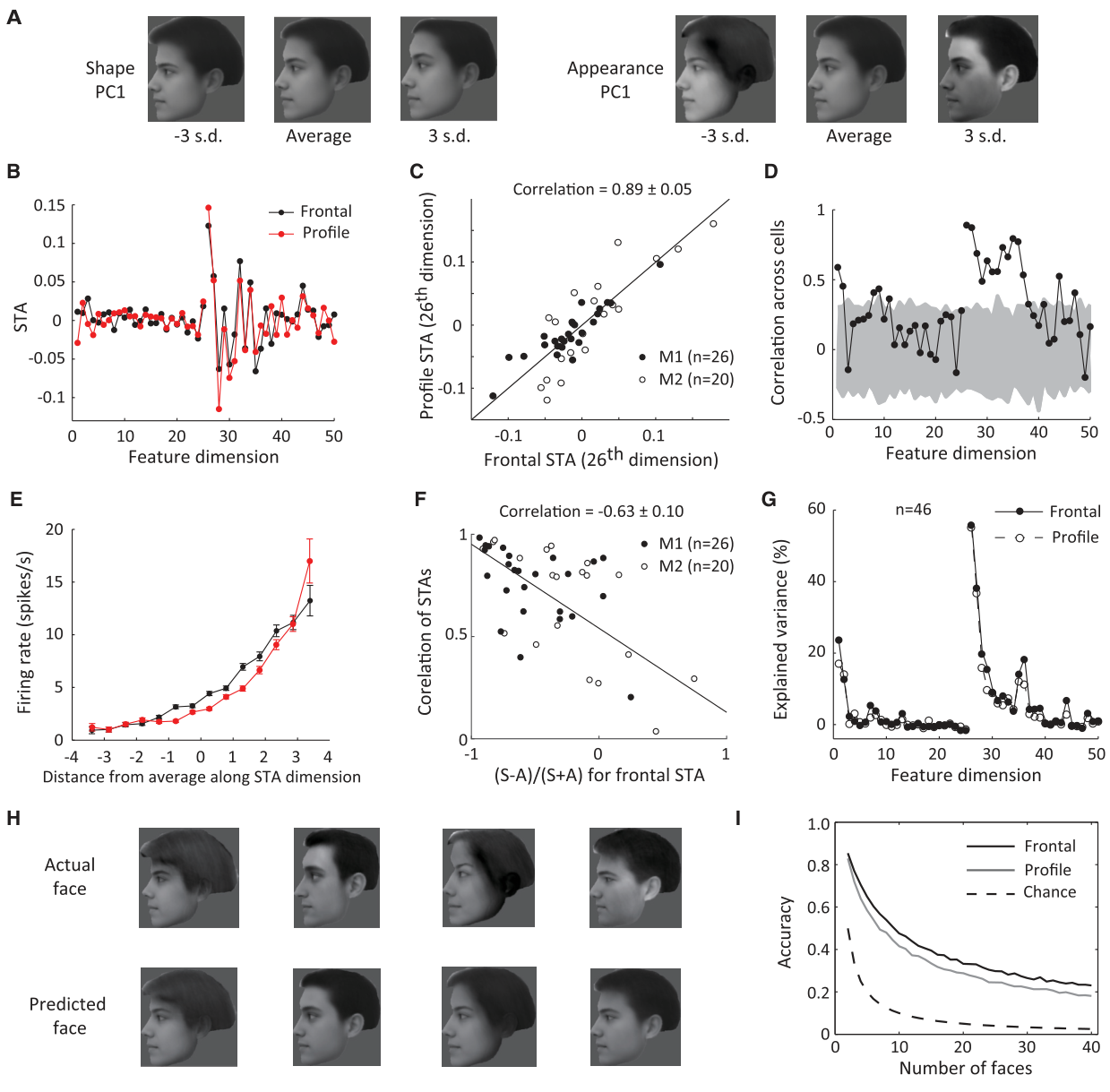
读图说明:(A) 构建共轭侧面面孔空间主成分;(B) 单个 AM 神经元在正面(黑色)与侧面(红色)刺激下计算所得 STA 向量的形态吻合;(C) 46 个神经元在第一外观维度上的跨视角 STA 相关性散点图;(D) 50 维特征上跨视角相关性分布,外观维相关显著超出置乱置信带;(E) 正面与侧面刺激下的斜坡调谐曲线;(F) 视角不变性与正面外观偏好呈正相关;(G–I) 利用基于正面面孔校准的线性模型成功完成侧面面孔的解码与图像重构。该图证实轴编码机制可延伸至跨视角表征,支撑主要结果第 5 条。
图 7 · 轴度量表征在识别任务上更灵活、高效、稳健
原文图注:Figure 7. An Axis-Metric Representation Is More Flexible, Efficient, and Robust for Face Identification (A) An axis metric can perform as well as a distance metric on an identification task for high-dimensional representation but not for low-dimensional representation. (A1) For an identification task, a linear classifier is usually non-optimal for a low-dimensional space (upper)... (A2) We explored how axis and distance metrics defined on feature spaces of variable dimensions perform in a face identification task. A simple network model (lower) was trained to identify one of the 200 faces based on 200 units with tuning defined by a distance metric or an axis metric... (A3) Error rate of identification was plotted against dimensionality for both models. (B) An axis metric is more efficient than a distance metric... (B2 and B3) Same as (A2) and (A3) but using ten input units. For high dimensionality, axis metrics outperformed the distance metrics. (C) Axis metrics are more distributed and more robust to noise than distance metrics. (C1) Weight matrices of networks in (B) after training using units defined by an axis metric or a distance metric (white indicates large weight)... (C2) Distributed inputs could help average signals with independent noise, resulting in high signal to noise (upper). The same network in (A2) was trained with noisy inputs (lower). (C3) Error rates of both models plotted against dimensionality. (D) The linear relationship between neuronal responses and facial features ensures diverse tasks can be performed. The gray disks indicate face space.
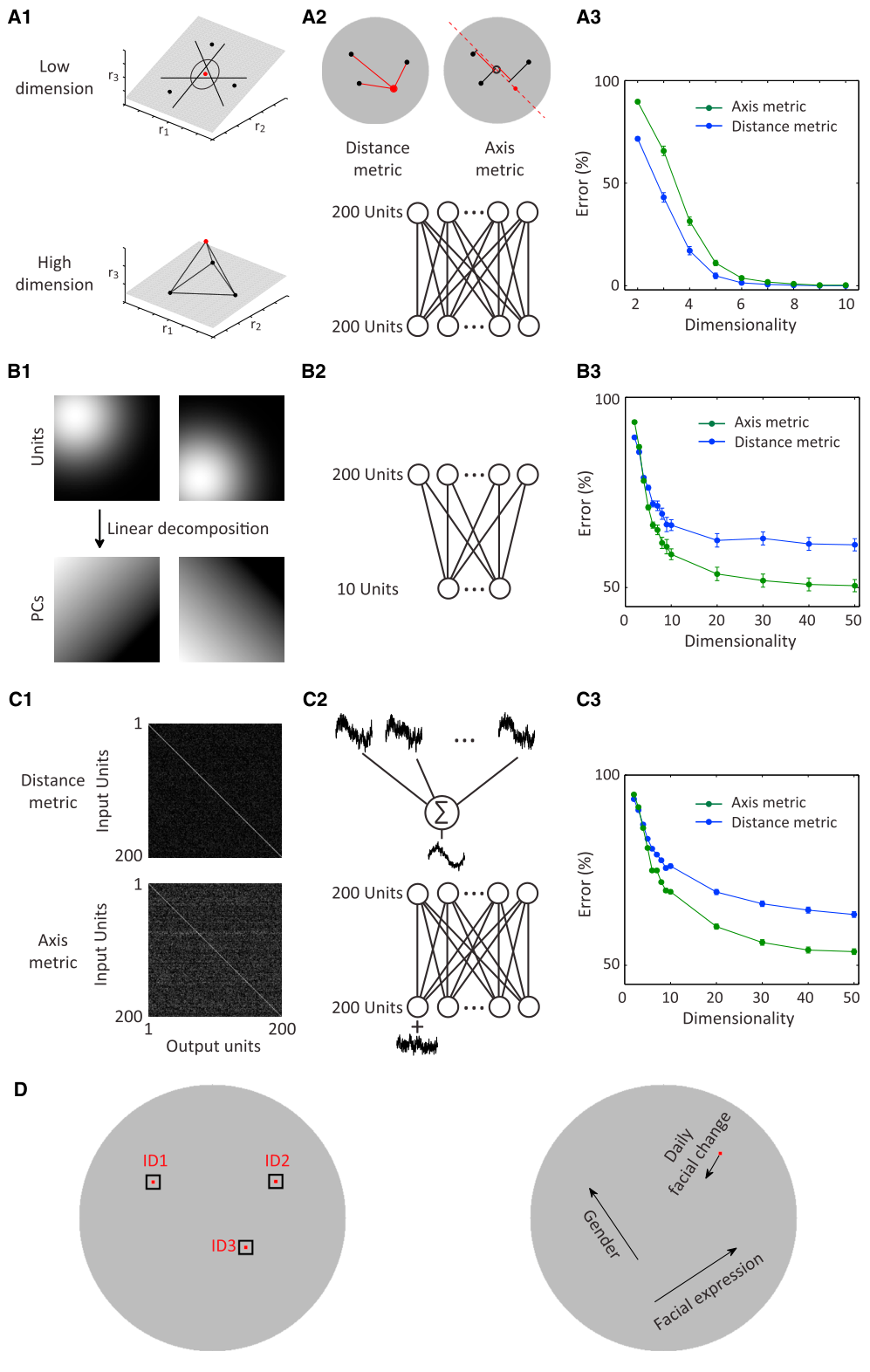
读图说明:(A) 二维低维空间中径向距离分类优于线性分类,但随特征维度扩增至 6 维以上,轴投影度量与距离度量的分类错误率趋同;(B) 在限制输入神经元规模(10 个单元)的条件下,高维轴模型分类表现显著优于距离模型,展现更高编码效率;(C) 权重矩阵热图表明距离模型连接权重高度集中于对角局部,而轴模型权重呈现分布式;在强噪声环境下,高维轴模型错误率显著更低,因分布式投影有助于平抑非相关神经噪声;(D) 线性轴编码支持下游网络根据不同任务目标灵活读出分类超平面。该图为主要结果第 5 条后半部分提供了计算理论论证。
讨论
作者指出,灵长类面孔加工网络并非存储具体个体图像的“样例记忆库”,而是由连续物理特征驱动的“正交坐标度量系统”。在具备生态有效性的形状-外观特征空间中,约 200 个神经元的放电模式足以双向实现面孔的高保真重构与放电率的高精度预测,轴模型对神经发放方差的解释率达到可解释测量天花板的 80.0%。在机制对话方面:研究复核并拓展了 Freiwald 等 (2009) 在卡通面孔中观察到的斜坡调谐现象,通过证明正交子空间内的调谐曲线平坦,确立了神经元执行一维线性投影而非局部径向距离计算的本质,排除了斜坡调谐与样例模型兼容的混淆;在计算涌现机制上,以视角不变分类为目标训练的深度卷积神经网络自发演化出轴式调谐与外观特征偏好,提示轴编码模式可能是前馈视觉层级网络应对高维客体分类任务的自适应解。作者同时指出了理论模型的边界:当前 50 维空间未包含动态微表情、发型变化及非人灵长类同种面孔特征;AM 轴表征对大范围物理遮挡与复杂自然光照变化的抗干扰能力仍有待后续验证;对于非面孔类的任意自然物体,由于缺乏同质性的解剖参考点,是否同样遵循低维连续轴表征,或依赖局部构型片段编码(Brincat & Connor 2004),需进一步探索;此外,IT 皮层内部仅实现面孔特征的高精度物理测量,而将特征转换为具体个体的决策性判定(如样例识别)更可能发生在下颞叶之后的下游脑区(如海马或内侧颞叶)。
一句话总结
本研究证实了灵长类大脑下颞叶面孔神经元遵循高维特征空间的线性轴投影编码原理:单个神经元的放电率正比于输入面孔在偏好特征轴上的标量投影,群体神经发放能够高精度线性重构任意人脸图像并实现跨视角泛化。这一发现排除了个体面孔表征依赖非线性“样例模板”的传统假说,确立了高级视皮层作为连续几何坐标测量系统的显式计算模型。