Object category structure in response patterns of neuronal population in monkey inferior temporal cortex

这篇文章用一次"大矩阵"式的测量回答了 IT 编码的老问题：给两只未受类别训练的猴子看 1084 张自然与人造物体图片，记录前部下颞叶皮层（inferior temporal cortex, IT）674 个神经元，结果发现刺激在群体反应模式（population response pattern）上聚出的簇，大体重现了人类直觉的类别层级——从"动物 vs 非动物"到"身体/手/脸"，再到"人脸 vs 猴脸"。作者进一步证明这种类别结构不是低级图像相似性的副产品，也不能从随机调谐的复杂特征模型单元中免费涌现，而且它由对类别反应并非最强的神经元共同承载——是"分布式类别表征"的代表性示范。

研究背景

人类影像学已经提示颞叶皮层存在对面孔、房屋、动物、工具等几类物体的类别化表征（Kanwisher 等 1997；Haxby 等 2001；Chao 等 1999），但这些研究普遍受限于刺激集小且可能有偏、并预先假定了类别结构。单细胞水平上，猴 IT 有面孔选择细胞已很确定（Bruce 等 1981；Desimone 等 1984），但这能否推广到其他类别无人知晓；受训把刺激分成几个任意组别的猴子在前额叶出现覆盖整类的单细胞反应（Freedman 等 2001、2002），人类内侧颞叶也有类别化的细胞（Kreiman 等 2000；Quiroga 等 2005）——可前额叶与内侧颞叶的物体视觉输入都来自 IT，而 IT 单个细胞看起来只表征单个刺激而非习得类别（Freedman 等 2003；Vogels 1999）。于是"类别表征在 IT 下游的多模态联合皮层"成了默认假设。缺口在于：从未有人在大量自然物体图像（而非任意的小刺激集）上、以群体（而非单细胞）为单位、不施加任何类别任务地检验 IT 是否自带类别表征。

研究思路

作者的核心策略是"数据驱动 + 无任务假设"。让猴子在被动注视下快速序列观看 1084 张彩色图片（每张 105 ms、无间隔，类似于自然扫视中的"一瞥"），把每个刺激在 674 个细胞上的平均反应组成一个模式向量，用两刺激模式间的 Pearson 相关（r）定义相似性、以 1−r 为神经距离（neural distance）——选相关系数的好处是只看群体反应的"模式"，自动折扣对比度、亮度等非特异性地改变整体放电率的因素。之后完全不让人类介入分类：先用多维标度（multidimensional scaling, MDS，含 Isomap 式非线性降维）把 1084 个刺激铺进低维空间，再用凝聚聚类（agglomerative clustering，平均连接）把神经距离连成一棵树；最后才拿人类惯例列出的 23 个直觉类别去"事后"给树的节点打分（节点得分 = 成员覆盖率 Ratio1 与纯度 Ratio2 的平均，用 Monte Carlo 随机分组估计机会水平，显著性要求得分超机会 4 个标准差且成员覆盖过半）。围绕这个主分析再铺四层验证：与低级物理相似性、模拟 V1 群体、HMAX 模型的复杂特征单元对比排除"平凡解释"；用线性感知机检验可读出性；用多种单细胞统计刻画表征的分布式性质；最后用第三只猴子的延迟匹配样本行为测试把神经距离与知觉距离挂钩。

方法

三只恒河猴（均为 2 只记录、1 只行为；猴子在进实验室前曾生活在人类家庭与动物园，接触过大量动植物与人造物——这一点对"自然类别"的解释很重要）。记录在两猴的前部 IT（猴 1 右半球 A15–20 mm，猴 2 左半球 A13–20 mm），覆盖上颞沟腹侧岸与腹侧凸面直至前中颞沟内侧岸，1 mm 间隔均匀推进、不按反应性质筛选，共 674 个隔离良好的神经元。刺激为灰底上的自然与人造物体彩色照片和绘画（长边 7° 视角），每细胞测试 1124±71 幅（中位数 1084）、重复 9±2 次；猴子须保持注视（±2°），每 1.5–2 s 给一次果汁。分析取刺激 onset 后 71–210 ms 的 140 ms 窗口，剔除前刺激污染严重的试次（约 15%）。每个细胞的反应向量先减去自身均值再按欧氏长度归一化（消除基线与动态范围的个体差异）；单细胞类别选择性用最低层 13 个类别检验（最优类别显著大于任何其他类别，Newman-Keuls P<0.05），并计算反应的"选择深度"式分布、次优类别间的 Wilcoxon 比较、以及仿 Haxby 等（2001）的"半类别相关"分析（每类随机对半分、跨全群体求相关，重复 1000 次）。行为实验用延迟匹配样本任务（44 张刺激、13–48 次重复/对，共 51806 试次、27 个会话），以非匹配试次的正确判别概率作为知觉距离。

主要结果

1. 群体反应模式自带类别簇：任意两刺激的群体反应相关在 −0.31 到 0.54 之间分布；动物类与非动物类刺激的反应模式呈负相关，动物类内部同一直觉类别内相关最高（图 2、3）。MDS 的二维投影就能看到脸、身体、手、非动物四个大簇，脸进一步分成人脸、猴脸、非灵长类动物脸，身体也分出亚群（图 4）；但 2D 投影只解释约 35% 的方差，提示真实结构在高维空间中。
2. 聚类树形式化地重现直觉层级（图 5，表 1–2）：第一分支就是动物 vs 非动物（得分均 0.92）；动物下分身体、手、脸；脸分灵长类与非灵长类，灵长类脸再分人脸与猴脸（人脸得分 0.98、猴脸 0.89、手 0.96、人身体 0.94）；身体一侧，人、鸟、四足动物的躯干聚在一起，鱼、爬行类、昆虫等低等动物自成一群。23 个直觉类别中多数动物类别及"汽车"（0.85）显著匹配，其余非动物类别（叶、花、水果、工具等）不匹配——与猴子生态相关性一致。两猴各自建树的类别得分高度一致（r=0.8，p<10⁻⁶）。
3. 排除平凡解释（图 6）：以像素颜色/亮度差、小波系数定义的物理相似性所建的树不出现类别；模拟 V1（Gabor 简单细胞 + MAX 复杂细胞）群体同样失败；HMAX 模型中调谐到随机 674 张图片的形状调谐单元（STU，含位置/尺度不变性）的群体反应模式也完全不聚出类别。因此类别结构是 V1 之后、且超越"随机复杂特征组合"的加工产物。作为可读出性的正面证据，674×10 的两层感知机用一半刺激训练后，对剩余刺激的分类正确率 86±3%（随机指派类别的对照仅 50±3%）。
4. 表征是分布式的（图 7–10）：255 个细胞（38%）对某一类别或类别组合显著最有反应（如人脸 54 个、人身体 36 个、手 26 个），但单个细胞对偏好类别与其他类别的反应分布大量重叠——即使面孔细胞也是如此（与 Tsao 等 2006 报道的后部 IT 近乎纯选择的面孔区形成对照）；把偏好同一类别的 10–20 个细胞的反应平均后，重叠基本消失。次优类别也携带信息：按类别反应排序后，约半数类别选择细胞能分辨排序差 5 的类别对（非选择细胞差 8 即可，图 9）；半类别相关分析显示，删掉对两类各自反应最强的细胞后类间仍可判别（如四足动物身体 vs 鱼），而把非最强细胞的反应打乱则相关显著下降（p=0.0002，图 10）。
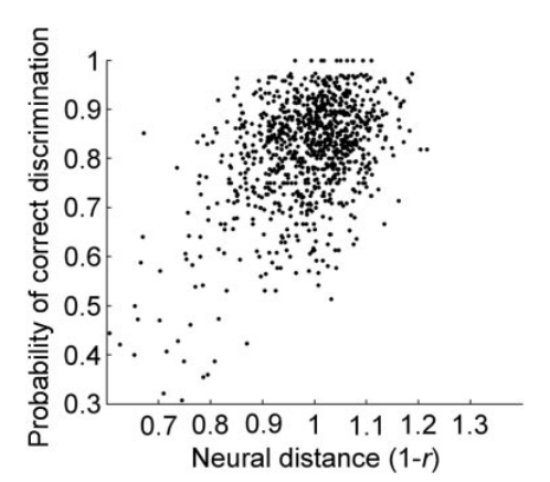
5. 局部小簇与行为对应（图 11、12）：空间距离 ≤1 mm 的细胞对反应相关更高，类别相关比刺激相关更强，但同类别细胞并不形成大片连续区域，而是散布为多个小簇；第三只猴子在延迟匹配任务中的混淆概率与 IT 神经距离显著相关（r=0.44，p<10⁻⁶），按判别率做的 MDS 显示猴子对动物物体的知觉类别结构与人类相似。

图注解读

图 1 · 记录部位分布

原文图注：FIG. 1. Positions of recording sites in 2 monkeys. Left: lateral views of the recorded hemispheres. Vertical lines indicate the anterior-posterior extent of the recording sites. Right: representative coronal sections. Recorded regions are indicated by gray. Recording sites were evenly distributed. ls, lateral sulcus; sts, superior temporal sulcus; amts, anterior middle temporal sulcus; rs, rhinal sulcus.

读法：左为两猴已记录半球的侧视（竖线给出记录位点的前后范围），右为代表性冠状切面，灰色标出被覆盖区域。要点是位点在 STS 腹侧岸与腹侧凸面均匀分布、不偏向任何反应类型——这为"结果来自无偏抽样"背书。

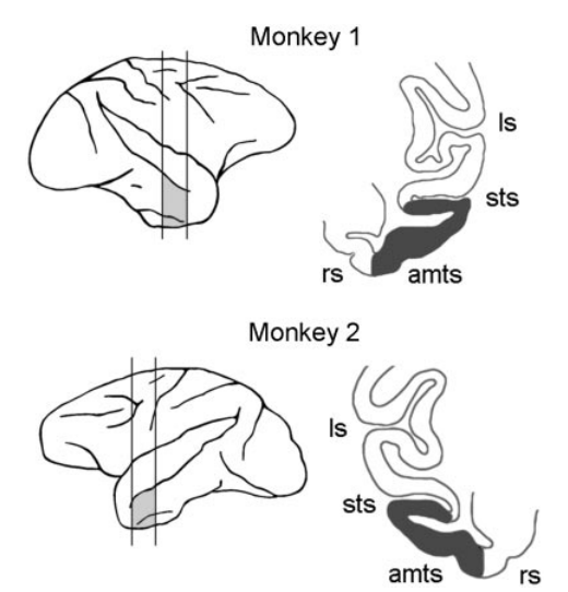
图 2 · 三个刺激对的群体反应模式相关示例

原文图注：FIG. 2. Examples of correlation between response patterns evoked in the 674 cells by 3 pairs of stimuli. F, 1 of the cells, and the x and y values of each F represent the normalized responses of the cell to the stimulus pair. The 3 pairs share a common stimulus, which is shown at the left. The Pearson's correlation coefficient (r) was 0.35, 0.20, and –0.20 for A–C, respectively. All 3 correlations are significant.

读法：三张散点图各画 674 个点，每点是一个细胞对"共享刺激 vs 比较刺激"的归一化反应；点云沿对角线的贴合程度就是两刺激群体反应模式的相似度（A 同类 r=0.35 > B 较远类 r=0.20 > C 异类 r=−0.20）。它用三个具体例子演示"类别越近、群体反应模式越像"这一全文的分析原语。

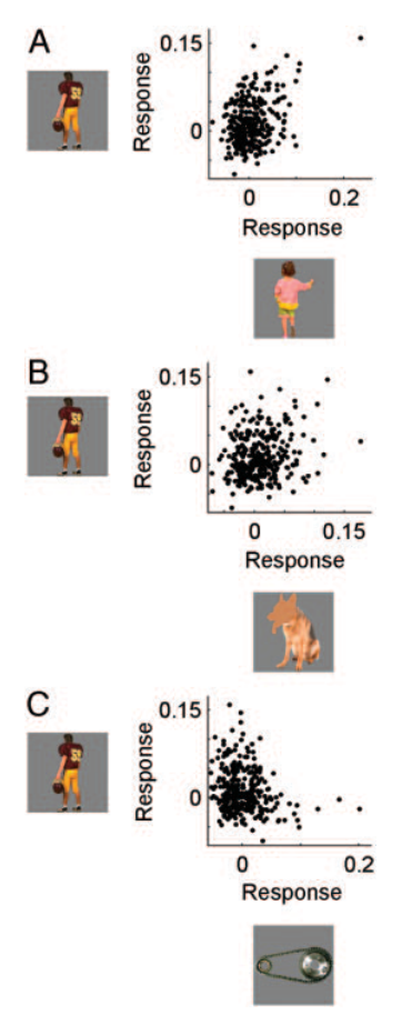
图 3 · 全刺激集两两相关的分布

原文图注：FIG. 3. Distribution of the correlation coefficients for the population response patterns. For each pair of the 1,084 stimuli, the correlation was calculated for the response patterns evoked by the 2 stimuli across the recorded cells.

读法：横轴是 1084 个刺激所有配对的相关系数（从 −0.31 到 0.54），纵轴是配对数。分布整体偏正且两尾都存在，说明群体反应模式有丰富的"远近"结构，而不是一刀切的相同/不同。

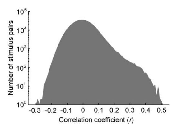
图 4 · 神经距离的低维投影（MDS）

原文图注：FIG. 4. Arrangement of the stimuli in a low-dimensional space based on multidimensional scaling (MDS) on the neural distances (1 – r) of the stimuli. Each point represents 1 of the stimuli. A–C represent 3 different projections of the space as denoted by the axis labels. All 1,084 stimuli are shown in A, whereas only faces and bodies are shown in B and C, respectively. The categories that are labeled here were found to have significantly matching nodes in the tree shown in Fig. 5.

读法：每个点一个刺激，点间距离近似神经距离。A 是全体刺激的投影，肉眼即可见脸、身体、手、非动物四个分离的簇；B、C 分别放大脸与身体，显示人脸/猴脸/非灵长类脸以及身体各亚群的分离。注意图注也提醒：这些标签只在树（图 5）中被判定为显著匹配的类别，且 2D 投影仅解释约 35% 方差——每张图只截取了高维结构的一个侧面。

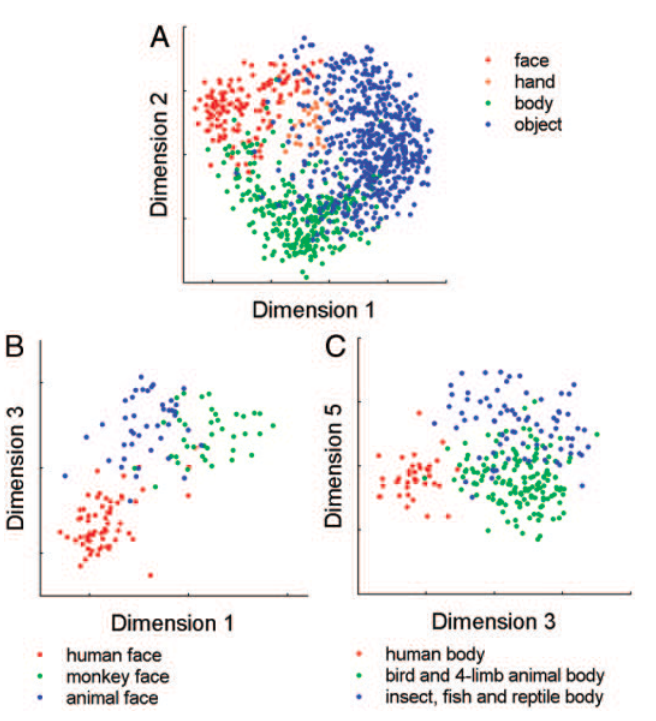
图 5 · 由神经距离重建的类别树

原文图注：FIG. 5. The tree reconstructed based on the neural distances. Red circles indicate the nodes significantly matching the categories. Blue circles indicate the nodes that had scores (see METHODS) significantly larger than chance score but included fewer than half of the category members. The blue nodes were added to indicate category combinations significantly matching the higher nodes. Five examples of category members are shown for each of the lowest-level categories, except for "other inanimate objects" (the rightmost node). The thirteen categories located at the lowest level are referred to as "the lowest-level categories" throughout this paper.

读法：这是全文的主结果图。第一分支为动物/非动物；红圈节点是显著匹配直觉类别的（得分超机会 4 SD 且成员覆盖过半），蓝圈是显著但覆盖不足一半的组合节点。沿树自右向左可以读出：动物→脸/身体/手→灵长类脸/非灵长类脸→人脸/猴脸；身体侧人、鸟、四足动物聚拢而鱼、爬行、昆虫另成一群。它把结果 2 的层级关系"画"了出来，并定义了后文单细胞分析所用的 13 个"最低层类别"。

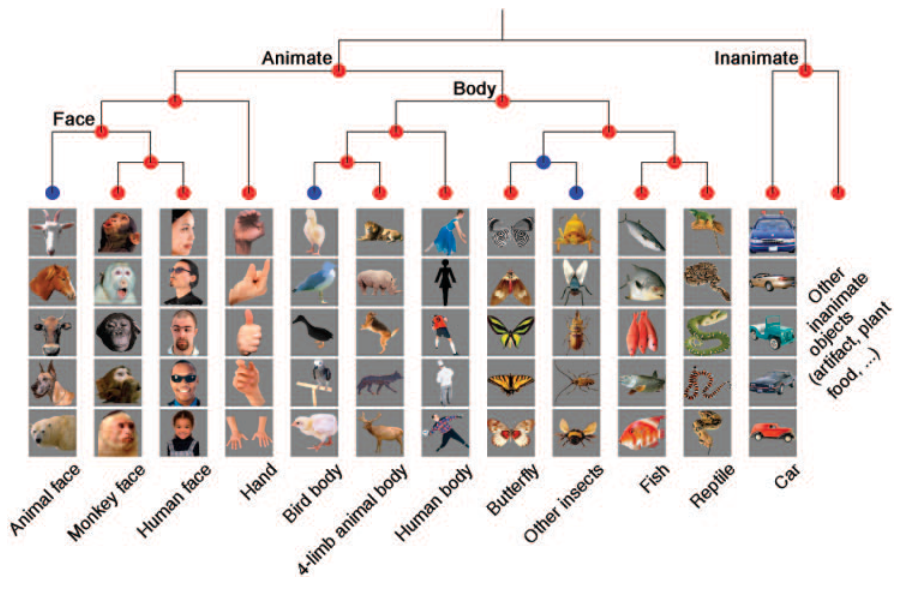
图 6 · 类别结构不来自低级相似性或模型单元

原文图注：FIG. 6. Object categories were represented by the responses of inferior temporal (IT) cell population but not by low-level image similarity or by model unit responses. A: average match of the intuitive categories with the best representative nodes of the trees formed by different distance measures (1). The match was quantified by the node score ((Ratio 1 + Ratio 2)/2), and averaged over all the significant categories of Fig. 5. △, expected scores for chance-level clustering of stimuli. Error bars represent SE. STUs, shape-tuned units in the HMAX model. These units were tuned to 674 stimuli randomly selected from the stimulus set. B: arrangement of the stimuli in the stimulus set according to MDS analysis on the response patterns of STUs did not replicate the clustering of stimuli based on the real IT cell population (compare with Fig. 4A). ……（截断）

读法：A 是关键对照柱图：真 IT 群体所建树的类别匹配得分远高于机会水平，而像素/小波物理相似性、模拟 V1 群体、HMAX STU 三种距离的柱子都落在机会线附近；B 给出 STU 群体的 MDS 投影，各类别混杂在一起（对照图 4A 的清晰分簇）。它支撑结果 3：类别结构是 IT 真实加工的产物，不是图像统计或随机复杂特征的副产品。

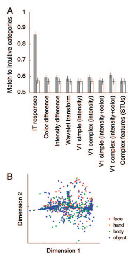
图 7 · 三个类别选择细胞的示例

原文图注：FIG. 7. Three examples of category-selective cells. Example responses to individual members of the preferred category (left), the averaged responses to the lowest-level categories (middle), and the magnitude of responses to individual stimuli of the lowest-level categories plotted against the normalized stimulus rank within each category (right) for a cell preferring human bodies (A), 4-limb animal bodies (B), and the combination of human bodies, 4-limb animal bodie, and bird bodies (C). Left and middle: horizontal bars indicate the stimulus presentation period. Middle and right: the best categories are shown in red. The categories that evoked responses significantly smaller than the best category but significantly larger than other categories (bird and reptile in B; reptile, fish, and other insects in C) are shown in blue. Gray indicates other categories. Normalized rank of 1 indicates the stimulus that evoked the largest response within the category.

读法：三列分别为单刺激反应（raster）、对 13 个最低层类别的平均反应、以及"幅度—类别内名次"曲线。A 细胞偏好人身体，B 偏好四足动物身体（蓝 = 次优但显著高于其他类，如鸟、爬行类），C 偏好人+四足动物+鸟的身体组合——即"类别组合"选择的活例。右列刻意暴露单个细胞反应分布的重叠：红曲线与灰曲线交错，为结果 4 的"单细胞并不纯净"埋下伏笔。

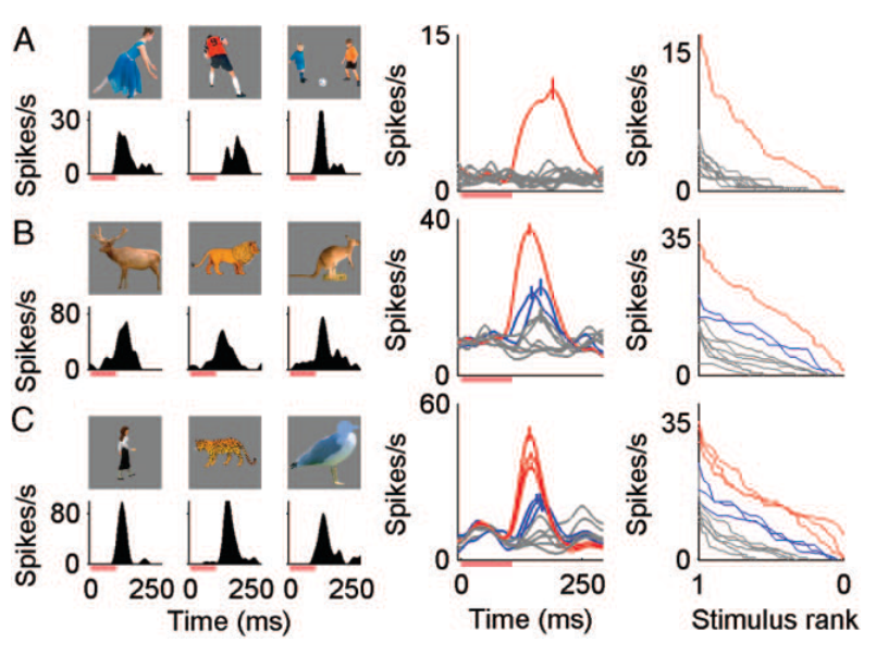
图 8 · 群体平均消除了单细胞的类别重叠

原文图注：FIG. 8. The overlap of average response magnitudes of stimuli in the preferred category (black lines) with responses to other stimuli (gray lines) for all the categorical cells (A) and for cells selective to human faces (B). A and B, left: mean responses to individual stimuli were normalized by the maximum mean response in each cell, and then responses to stimuli of the same normalized rank were averaged across cells. Normalized rank of 1 indicates the largest response in the stimulus group. A, right: normalized mean responses to the same stimulus were averaged over 10–20 cells preferring the same category in each monkey (performed for monkey faces, human faces, human bodies, or hands). The resulting magnitude-rank curves were then averaged across categories and monkeys for the figure. B, right: similar to A but the normalized mean responses to individual stimuli were averaged among 11 or 20 cells selective to human faces in each monkey. ……（截断）

读法：左列是"所有类别选择细胞"的合并曲线：黑（偏好类别）与灰（其他）分布大面积重叠；右列把偏好同一类别的 10–20 个细胞先平均再做同名次曲线，黑灰几乎分离开。即使只看人类面孔细胞（B）也是同样模式。此图以最直观的方式支撑结果 4 前半：类别信息靠"同类细胞互补平均"而变得纯净。

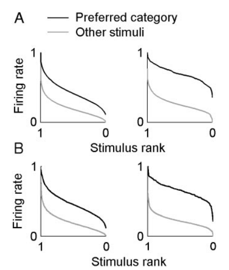
图 9 · 次优类别反应也携带类别信息

原文图注：FIG. 9. Many IT cells showed significant differences in their responses to suboptimal categories. For each cell, the lowest-level categories were ranked based on the average response magnitude, and the significance of difference in response magnitudes was calculated for each pair of category ranks (Wilcoxon test, significance defined as P < 0.05). Individual trial responses pooled for all the stimuli belonging to each category were used for the comparison. The proportion of cells that showed a significant difference for each category-rank pair is color-coded for the 255 category-selective cells (A) and the remaining 419 cells (B).

读法：横纵轴都是类别名次（1 为该细胞反应最强的类别），颜色编码"该名次组合间反应差异显著"的细胞比例。沿对角线越远的格子颜色越深：对 255 个类别选择细胞，名次差 5 时约 50% 细胞显著（A）；其余 419 个细胞名次差 8 才达到同样比例（B）。它支撑结果 4 后半：即便在非最强类别上，IT 神经元仍在做类别分辨。

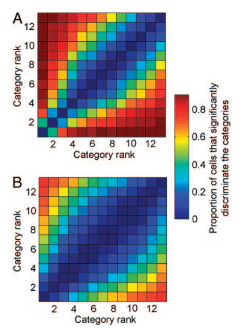
图 10 · 半类别相关：删掉最强细胞仍可判别类别

原文图注：FIG. 10. Within- and between-category correlations of population response patterns. Each lowest-level category was randomly divided into 2 halves, and mean responses of every cell to each half were calculated. The correlation of the mean responses across the population of cells was calculated for all possible pairs of categories (n = 91). The procedure was repeated 1,000 times with different random divisions of the categories, and the mean value of correlation coefficient was obtained for each of the category pairs. △, correlations calculated over the 674 cells. 1, correlation coefficient calculated after excluding the cells maximally responding to either of the paired categories. ■, correlation coefficient for all the cells but after shuffling of the responses for the cells that did not respond maximally to either of the 2 categories. Error bars represent 95% confidence interval. ……（截断）

读法：矩阵中每个格子是一对类别的群体反应相关（对角线为类内自相关）。三种记号对比：全 674 细胞（△）类内相关明显高于类间；删掉对两类各自反应最强的细胞后（1）类内仍高于类间——例如四足动物身体与鱼在没有各自"专家"细胞的情况下仍可分开；而把非最强细胞的反应打乱（■）则相关显著削弱（p=0.0002）。这是结果 4 中"分布式"论断的决定性证据，方法上直接呼应 Haxby 等（2001）的人脑 fMRI 分析。

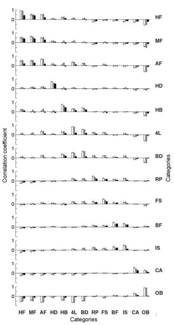
图 11 · 相近细胞的反应相关随距离衰减

原文图注：FIG. 11. Response correlations for pairs of cells with various distances from each other. The Pearson's correlation coefficients were calculated based on mean responses to the 1,084 individual stimuli (left) or based on averaged mean responses to the lowest-level categories. Distances between recording sites were divided into 11 bins, and the correlation coefficient was averaged over cell pairs within each distance bin. The averaging was performed separately in each monkey. Error bars represent s.e.m. Note that, unlike the neural distance, which was based on the response correlations for stimulus pairs across the neural population, this analysis is based on the response correlation for cell pairs across the stimulus set.

读法：横轴是记录位点间距（11 个分箱），纵轴是细胞对的反应相关（左按单刺激、右按类别平均）。曲线在 ≤1 mm 处最高、随后迅速降低并在 1 mm 后趋平；类别相关（右）整体高于刺激相关（左）。图注特别提醒这与"神经距离"是两个正交的量：前者是细胞对在刺激集上的相关，后者是刺激对在细胞群上的相关。此图支撑结果 5 的空间部分：局部相似的小簇而非大块连续拓扑。

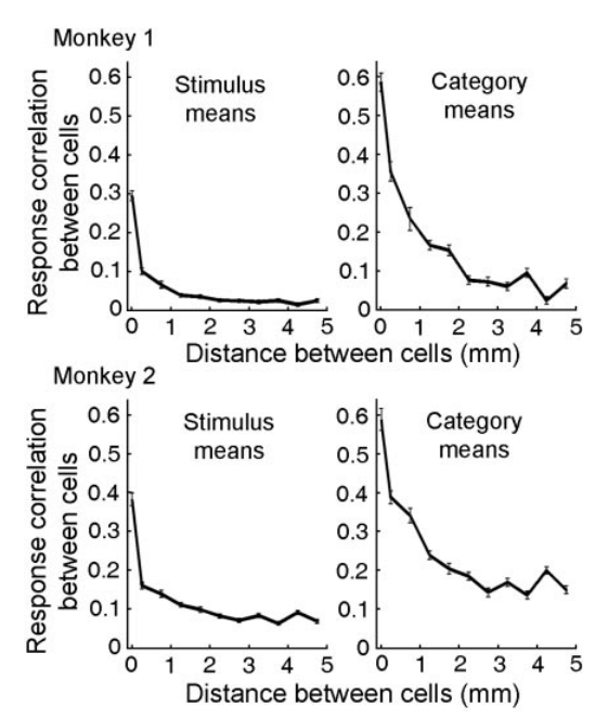
图 12 · 行为判别率与 IT 神经距离相关

原文图注：FIG. 12. Probability of correct discrimination of stimulus pairs in a delayed matching-to-sample task plotted against the neural distance of stimulus pairs. A 3rd monkey performed the task with 44 stimuli selected from the stimulus set.

读法：散点图的横轴为刺激对的 IT 神经距离（1−r），纵轴为第三只猴子在延迟匹配任务中对该对的正确判别概率（=1−混淆概率）；两者正相关（r=0.44，p<10⁻⁶）。也就是说，IT 反应模式里"离得远"的两张图，猴子在行为上也更不容易认混。此图把神经侧的类别结构与动物的知觉行为接通，支撑结果 5 的行为部分。

讨论

作者的解释分三层。第一层是主张本身：IT 群体反应模式重建了直觉类别及其结构，而且整个流程是数据驱动的——MDS 与聚类都不需要预先指定类别结构，直觉类别只用于事后打分；与 Hung 等（2005）"从 IT 读出预定义类别"相比，这里进一步证明了"内在的"类别表征同时包括各单个类别与它们之间的直觉关系。第二层是分布式机制的刻画：约 40% 的细胞有显著类别选择性，但单细胞反应分布重叠大，10–20 个同类细胞的平均即可消除重叠（不同细胞的刺激—类别错配方式不同，因此互补），而具有相似类别选择性的细胞又恰好在皮层上局部成簇，于是"按皮层位置汇总"就成了把信息读出的可行方式；次优类别的反应则支撑起多层级同时分类（一张人脸可同时靠最强反应归入人脸类、靠次强反应归入大类、靠动物类细胞的反应归入动物类），并被作者认为可能构成层级类别系统的知觉基础。第三层是"类别结构如何从特征选择性中涌现"：随机选取复杂特征的模型单元失败，说明 IT 并非随机挑特征，而可能按猴子行为之需选取特征——类别判别或许正是塑造其特征选择性的因素之一，这种适应可能经由后天经验与演化实现。作者也坦陈限制：并不假设猴子拥有树上全部类别（"汽车"很可能没有），但 Sands 等（1982）与本文的行为测试说明猴子至少拥有与人相似的部分动物类别结构；每半球 322/352 个细胞的样本不足以对类别表征拓扑下强结论，且图 11 的分析假设簇为球形；快速序列呈现范式无法评估晚于测量窗口的反应的影响。

一句话总结

这是"群体码讲类别"的范本之作：无训练、被动注视、千张图片、六百多个细胞，让类别结构自己从数据里长出来，再用物理相似性、模拟 V1、HMAX 三个对照组把"这是不是显然的"逐个否掉。我特别欣赏图 10 那组半类别分析——它把"类别码分布在专家细胞之外"从一个口号变成了可删减、可打乱验证的量化事实；至于猴子究竟"拥有"哪些类别、以及猴 IT 缺少工具/家具类表征是人猴差异还是刺激集问题，文中自己也没有下定论，我读后也倾向于把它当作开放问题而非定论。