这是一篇方法学论文,针对功能连接分析中的信息压缩问题:多数连接指标先把 ROI 内的多体素活动模式压缩为单一数值(均值或主成分),再计算相关。作者反其道而行之,使用交叉验证的岭回归在体素对体素维度直接估计两个 ROI 之间的线性变换矩阵,并为该矩阵定义三个可解释指标:拟合优度(goodness-of-fit, GOF)、稀疏度(sparsity)与模式形变(pattern deformation)。研究采集 4 名被试的事件相关 fMRI 数据进行概念验证,考察早期视觉皮层(EVC)向 ITC、FFA、PPA 三个高级视觉区的模式变换,将功能连接从标量相关系数扩展为具备几何特性的映射矩阵。
研究背景
功能连接分析常先把一个 ROI 内的多体素活动压缩为平均时间序列或主成分,再计算脑区间相关。这一做法虽然能得出明确的标量连接值,却无法反映输入区的空间活动模式如何映射为输出区模式。若两个区域各自保留不同的表征结构,仅比较平均活动难以判断它们是共享同类信息,还是一个区域的模式被系统性变换为另一个区域的模式。已有的多体素方法或侧重表征相异度距离,或预先经主成分分析降维,仍无法直接刻画映射的稀疏性与几何形变。
线性估计虽不能覆盖真实的全部非线性神经加工,但提供了可解释的基准模型。岭回归可以在未降维的体素空间中估计变换矩阵,并由交叉验证评估泛化性能。该矩阵可从三个维度进行解释:解释输出方差的比例、是否主要由少数体素连接主导,以及奇异值谱是否对不同方向进行非均等缩放。由于岭回归的平滑正则化不会将不重要参数精确置零,稀疏度无法通过直接统计零元素获得,必须结合噪声水平由蒙特卡洛模拟校准;形变指标同样需要校准,以避免把噪声造成的奇异值谱衰减误判为生理特征。
Basti 等据此提出多体素模式变换分析框架,并使用 EVC 至 ITC、FFA、PPA 的事件相关 fMRI 数据进行概念验证。研究旨在评估原始体素空间中的线性映射是否显著、是否保留类别偏好、映射是否稀疏,以及不同靶区的形变特征是否存在差异。结果表明,线性模型能够解释部分方差并复现部分类别结构,使皮层间连接得以进行几何分析。受限于 4 名被试的样本量、预设的前馈方向以及线性假设,实证结果主要用于方法和指标验证,尚不能作为确立的生理连接定论。
研究思路
研究采用“线性估计模型 + 模拟校准 + 真实数据验证”的流程。作者将模式映射形式化为 Y = TX + E:X 与 Y 分别表示输入区与输出区的模式矩阵(各列对应各刺激条件的 beta 估计值),T 为待估变换矩阵,E 为残差。研究选用岭回归(ridge regression)而非普通最小二乘或 LASSO:岭回归能够提供唯一且数值稳定的平滑解,但估计所得矩阵元素均不严格为零。因此,稀疏度无法通过数零直接计算,需由蒙特卡洛模拟在已知稀疏度和噪声水平下建立参照曲线,再将实测数据投影至“衰减率 × 拟合优度”平面完成推断。三个指标与线性代数几何概念相对应:GOF 对应交叉验证的解释方差百分比;稀疏度对应变换矩阵中有效零元素占比(与地形图投射及拓扑投射相联系);形变对应变换矩阵的奇异值谱——根据极分解定理(polar decomposition),任何方阵线性变换均可分解为正交旋转/反射矩阵与对称缩放矩阵,奇异值即为各主轴方向上的缩放因子。全流程旨在使这三个几何特征能够在含噪 fMRI 数据中稳健定量。
方法
数据来源于既有公开发表的数据集:4 名健康受试者(平均年龄 35 岁,2 名女性),观看 96 张呈现在灰色背景上的孤立物体彩色图片(175×175 像素),包含 24 张面孔、8 张场景,以及人体、自然物和人造物体。刺激视角为 2.9°,每次呈现 300 毫秒,刺激间隔 3700 毫秒,被试在扫描中执行注视点颜色变换检测任务;每张图片在每个 run 呈现一次,每位被试在两个不同日期的 session 中各完成 6 个 9 分钟的 run。另包含独立的 block 设计定位实验(灰度面孔、物体、场景图片,30 秒 block,5.7° 视角,one-back 任务)用于定义感兴趣区。扫描采用 3T GE HDx 磁共振系统与 16 通道线圈,体素尺寸 1.95×1.95×2 mm³,TR 2 秒,每个 run 采集 272 个全脑体积,25 层轴位覆盖双侧下颞皮层(ITC)与 EVC。预处理基于 BrainVoyager QX 1.8 在个体原生空间完成(未做 Talairach 变换),FFA/PPA 基于 4 mm 平滑数据定义,EVC/ITC 基于未平滑数据定义。单张图片的响应幅度由体素单变量通用线性模型估计,设计矩阵包含 96 种刺激的血氧动力学预测器,以及头动参数、线性漂移和傅里叶基底等协变量。
ROI 依据独立定位数据勾画:FFA 为梭状回内基于“面孔减场景与物体”对比、从峰值体素迭代生长的连续体素簇,每半球各 128 个体素;PPA 基于“场景减面孔与物体”对比、从海马旁回峰值体素以相同规则生长,每半球各 128 个体素;ITC 选取皮层掩模内视觉响应最强的 316 个体素(双侧),EVC 选取双侧距状沟周围解剖范围内响应最强的 224 个体素(EVC 与 ITC 不要求体素连续)。三个指标的计算方式如下:GOF 定义为输出区模式总方差中被交叉验证线性变换所解释的百分比(GOF = 100(1 − Λ(λ)/(NY·Ns))),显著性采用 10000 次刺激标签随机置换结合 Kolmogorov–Smirnov 检验(p < 0.05);岭回归正则化参数 λ 采用留一刺激交叉验证确定,并推导了降低计算复杂度的解析算法。稀疏度计算先将估计矩阵按最大绝对值归一化,定义阈值以上元素比例随阈值变化的密度曲线 d(P),拟合其指数衰减参数 b 作为衰减率(RDD),随后进行蒙特卡洛模拟:以实测 EVC 模式作为输入,设置 6 档真实稀疏度(50%–99%)与 10 档噪声强度(γ 0–0.9),各重复模拟 1000 次,将实测 RDD–GOF 坐标置于参照曲线族中插值推断真实稀疏度。形变指标同理:提取变换矩阵的奇异值谱,拟合指数衰减率 RDSV,基于 4 档衰减率(0、−0.01、−0.1、−1)完成蒙特卡洛校准。真实数据采用跨 session 交叉验证(session 1 估计、session 2 测试,反向重复后取平均),以消除两区域间非刺激相关的内在自发生理波动带来的虚假相关。
主要结果
- EVC 与三个高级视觉区之间均存在统计显著的线性模式变换关系,其中与 ITC 的拟合优度最高(图 4)。以全部 96 种刺激计算,EVC→ITC 的 GOF 最高且跨 session 保持稳定(26.9±6.4 与 27.8±7.6),显著高于 EVC→PPA(p = 0.001,配对 t 检验,Cohen's d = 5.97);EVC→FFA 居中(14.2±3.7 与 16.8±5.9),与 ITC 的差异未达显著水平(p = 0.066,d = 1.41);EVC→PPA 最低(6.6±4.3 与 8.8±4.2)。
- GOF 表现出与脑区偏好一致的类别特异性(图 4 与补充材料 S4 图)。仅针对 24 张面孔刺激时,EVC→ITC 显著高于 EVC→PPA(p < 0.001,d = 7.41),EVC→FFA 亦显著高于 EVC→PPA(p = 0.007,d = 3.31);仅针对 8 张场景刺激时,仅 EVC→ITC 与 EVC→FFA 差异显著(p = 0.010,d = 2.95)。单刺激分析显示,FFA 与 ITC 在有生命物体上的 GOF 系统性升高(FFA 中 38/48 张高于全部刺激均值;PPA 相反,39/48 张有生命物体低于均值、35/48 张无生命物体高于均值,Fisher 精确检验均 p < 0.001),表明线性映射能够捕捉各靶区特异偏好的类别信息。
- 由 EVC 经线性预测重建的高级区表征结构保留了部分真实几何特征(图 5)。基于预测模式构建的相异度矩阵与真实 RDM 下三角的相关系数(LPRD 值)分别为 ITC 0.19、FFA 0.16、PPA 0.15(均 p < 0.001);部分特征性类别块结构(灰框标注的 ITC 与 FFA 块)在预测矩阵中依然可见,但整体表征信息存在衰减。
- 估计所得变换矩阵具有显著稀疏性,但未达到严格的一对一拓扑映射水平(图 6)。三对投射的稀疏度估计均大于 80%:EVC→PPA 最高(>90%),EVC→FFA 与 EVC→ITC 介于 80%–90% 区间。理论上,若两区域各 200 个体素之间实现严格的一对一映射,稀疏度需高于 99.5%;实测结果更符合一对少数体素(one-to-few)的发散或会聚投射。各估计值在被试间的标准误相对较大。
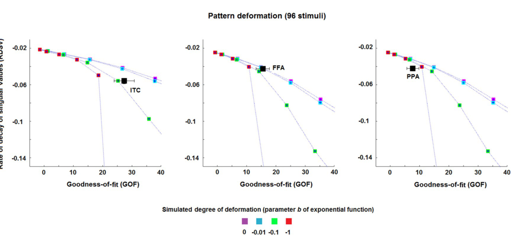
- 不同映射路径对输入模式的几何形变程度存在分离(图 7)。EVC→FFA 的衰减参数落在 0 至 −0.01 曲线区间,形变接近各向均匀(近乎刚性旋转加均匀缩放);EVC→ITC 的衰减参数约为 −0.1,EVC→PPA 低于 −0.1,两者对不同特征维度的模式施加了显著差异化的放大或抑制。补充分析显示,最优正则化参数 λ 与 GOF 呈显著负相关(r = −0.86,p < 0.001),10 折交叉验证获得了一致结论。
图注解读
图 1 · 方法框架总览:从模式矩阵到三个指标
原文图注:Fig 1. The purpose of the current study is 1) to describe a computational approach for estimating linear transformations T between MV-pattern matrices X and Y (each matrix column contains the beta-values associated with a different stimulus type) of two ROIs, and 2) to derive three novel connectivity metrics describing relevant features of those functional mappings.
该示意图展示整体分析流程:左侧为输入区 ROI 的模式矩阵 X,右侧为输出区的模式矩阵 Y,各列为不同刺激(96 种条件)的逐体素 beta 估计值;中间的变换矩阵 T 经岭回归求解;模型随后引出 GOF、稀疏度与模式形变三个指标。刺激维度(列)在变换中保持对齐,体素维度(行)实施映射,表明该方法并非分析时间序列共变,而是直接建模表征空间之间的空间结构对应。
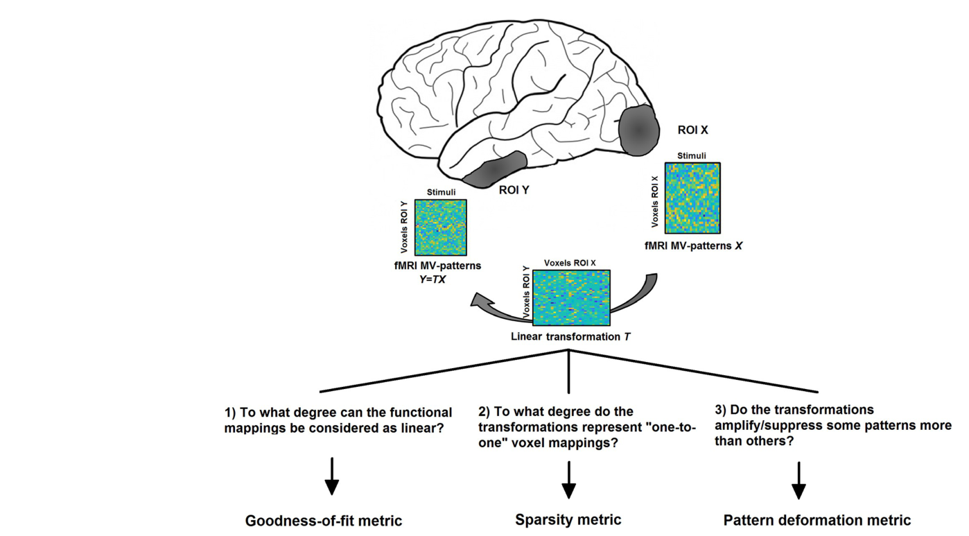
图 2 · 稀疏度指标的模拟校准
原文图注:Fig 2. Estimation of the percentage of sparsity using a ridge regression method. A) An example of a simple sparse simulated transformation: 90% of the entries are equal to 0, while the other 10% of the entries are equal to 1. B) Estimate of the transformation in A obtained by using the ridge regression method. The lighter background indicates that the estimated elements are different from zero even if in the original transformations they are exactly equal to zero. C) Density of the thresholded estimated transformations, i.e. the percentage of matrix entries that exceed the threshold, as a function of the threshold. In this toy example, we generated 30 realisations for four simulated percentages of sparsity (0%, 50%, 80% and 90%). D) Density of the thresholded estimated transformations associated with a degree of sparsity of 90% and different GOF values (i.e. different levels of noise in the model). E) Scatter plots of the rate of decay of the density curves (RDD) shown in panel C against goodness-of-fit GOF for the 30 simulation realisations of each of the four different cases. It is evident that simulated transformations of e.g. 90% sparsity are associated with a certain range of RDD and GOF values (red dots) which, at least for sufficiently large values of GOF, are different from those related to transformations with 80% of sparsity (green dots).
五个面板说明岭回归下稀疏度估计需结合模拟校准的原因。A 为模拟真值矩阵(90% 元素为 0,其余为 1);B 为岭回归估计结果,原本为零的位置被赋予平滑非零数值(浅色背景),反映 L2 正则化对绝对稀疏结构的平滑效应;C 展示不同真实稀疏度下密度曲线的衰减趋势(稀疏度越高,曲线下降越陡峭);D 表明同一真实稀疏度下,噪声增强会导致曲线衰减放缓,单一密度曲线无法区分“高噪声下的高稀疏”与“低噪声下的低稀疏”;E 给出校准方案:将曲线衰减率 RDD 与 GOF 联合投影至二维散点平面,不同稀疏度在不同噪声水平下均形成可分集群,为后续图 6 提供了定量参考。
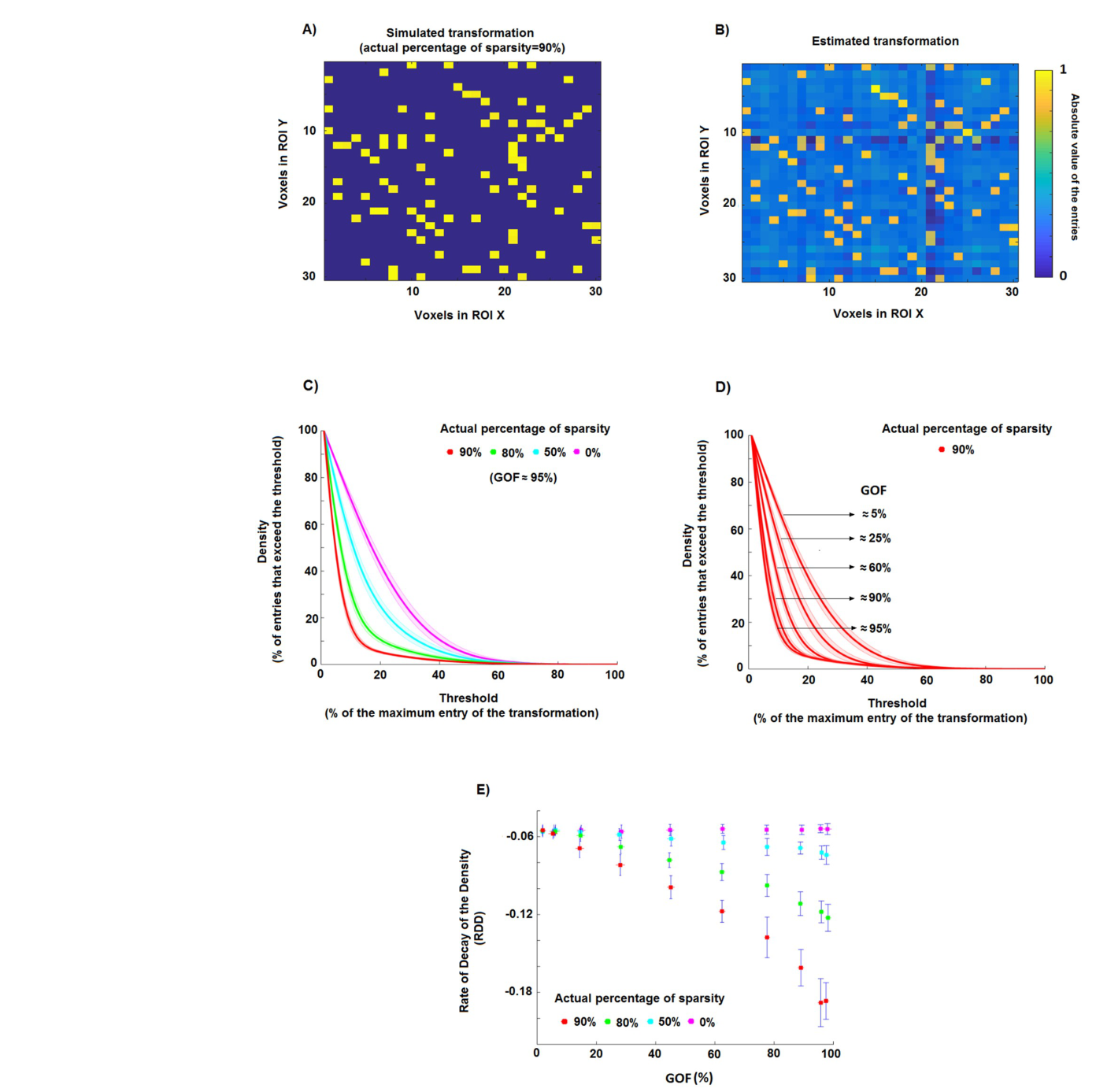
图 3 · 形变指标的几何含义与校准
原文图注:Fig 3. Estimation of the pattern deformation. A) A geometric interpretation of a linear pattern transformation between patterns of equal dimension. Two MV-patterns of two ROIs, let us say EVC and ITC, can be seen as two points of two vector spaces, and the matrix transformation T between them can be seen as a linear mapping between these two vector spaces. In this panel, a sphere (representing for simplicity the MV-patterns of EVC for a set of stimuli) is transformed by T into the ellipsoid (representing the ITC MV-patterns for the same set of stimuli). The singular values (SVs) of T are important features of this mapping. For example, if the number of voxels is the same in both ROIs, the SVs (μ values in the Fig) describe how much the EVC pattern is deformed by the transformation. For instance, constant values across all SVs can indicate an orthogonal transformation, that is, a linear mapping in which the ITC pattern can be completely described as a rotation (or reflection) of the original EVC pattern. B) The curves of the SVs (a monotonically non-increasing function with b as the rate of decay) of the estimated transformations for four different simulated rates of decay (b = 0, −0.01, −0.1, −1). C) The curves of the SVs of the estimated transformations associated with orthogonal transformations (i.e., b = 0) and different GOF values (i.e. different levels of noise in the model). D) Scatter plot between goodness- of-fit GOF and the rate of decay of singular values RDSV, i.e. the estimated decay obtained by fitting an exponential curve to the SVs of the estimated transformation for the four different cases. By using both the RDSV and GOF, it is possible to characterise the different induced pattern deformations, even if the level of noise is not equal to 0%.
A 面板呈现模式线性变换的几何示意:球体经变换矩阵 T 映射为椭球体,奇异值 μ 代表各主轴维度的缩放比例;奇异值大小均等对应正交旋转或反射,奇异值快速衰减则表明特定维度的表征模式受到强烈压缩。B 展示四档设定衰减率(0、−0.01、−0.1、−1)下的奇异值谱衰减形态;C 说明测量噪声会导致估计出的奇异值谱形态趋于扁平;D 通过将 RDSV 与 GOF 结合在二维坐标系中,使不同程度的几何形变在存在测量噪声时依然可分,作为图 7 读数的判定基准。
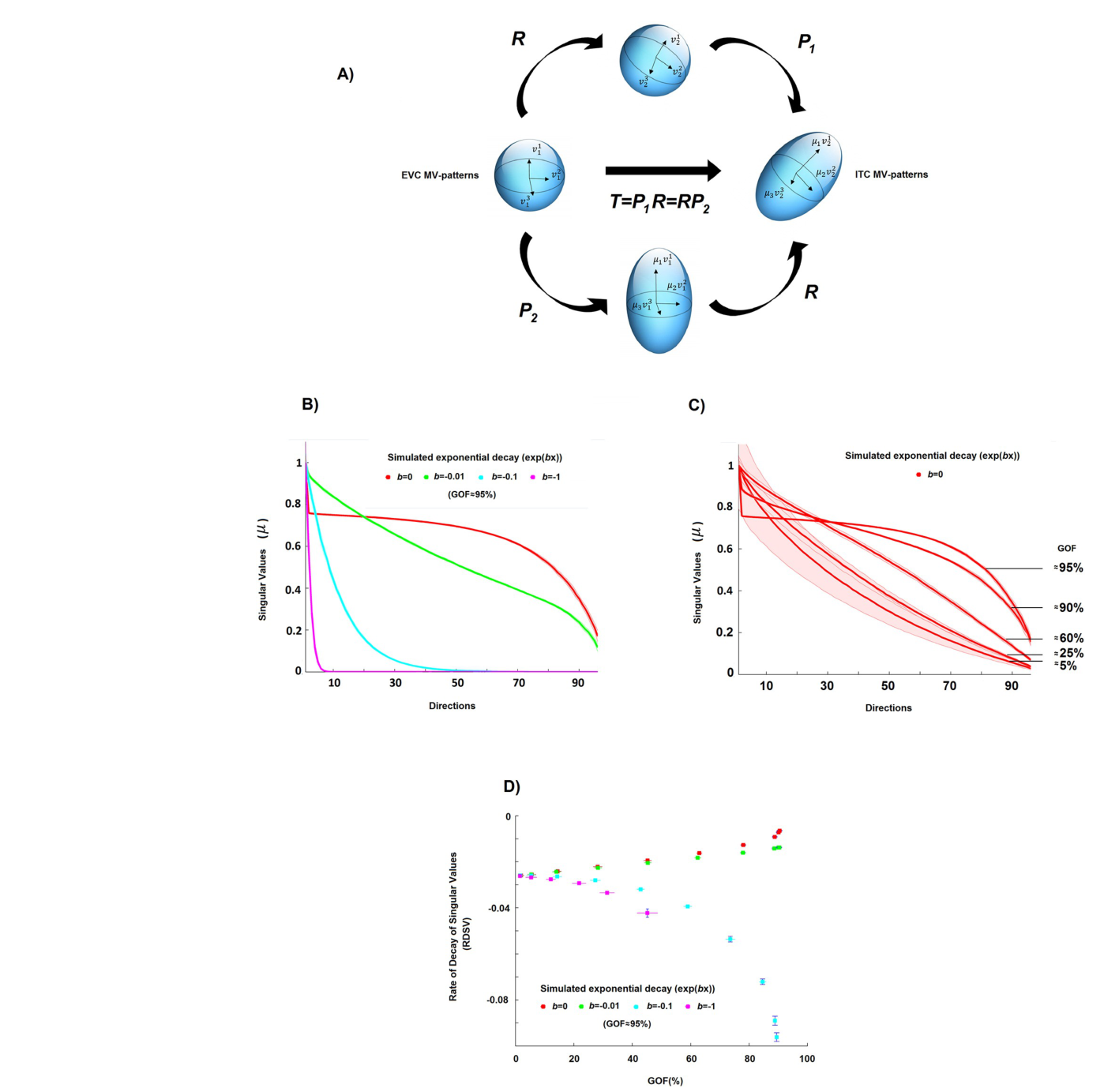
图 4 · GOF 的主结果与类别子集
原文图注:Fig 4. The goodness-of-fit (GOF) values for all the subjects and sets of stimuli. A), B) and C) The percentages of GOF by using the linear pattern transformations from EVC to the three output ROIs for all 96 stimuli, the 24 face stimuli and the 8 place stimuli, respectively. The p-values for the paired t-tests are reported even if based on only four subjects.
三个面板分别呈现基于全部 96 种刺激、24 张面孔及 8 张场景计算所得的各路径 GOF(横轴为三对脑区映射,纵轴为解释方差百分比,散点对应各被试)。A 面板中 EVC→ITC 的 GOF 显著居首,FFA 居中,PPA 最低;B 面板中 EVC→PPA 在面孔刺激下的 GOF 大幅下降,体现出 PPA 对面孔表征解释力的缺失;C 面板中场景刺激的整体 GOF 均偏低,仅 ITC 与 FFA 之间差异达到显著。图注注明配对 t 检验统计量基于 4 名受试者,需注意小样本局限。
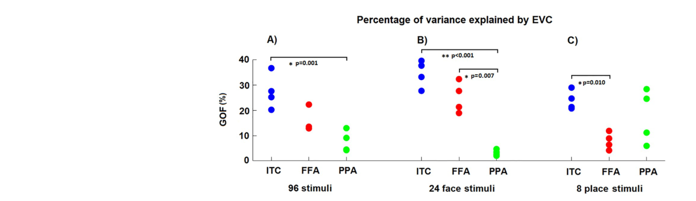
图 5 · 用 EVC 预测出的表征相异度矩阵
原文图注:Fig 5. Representational dissimilarity matrices for actual and estimated patterns. Left panels: percentile of the dissimilarity (correlation distance) among the multivariate patterns of the actual ITC, FFA and PPA. Right panels: percentile of the correlation distance among the estimated patterns from EVC. The estimates of the multivariate patterns were obtained by using the pattern transformation between EVC and ITC, FFA and PPA. While some information is lost, some characteristic patterns which are visible in the left panels (e.g. the patterns highlighted by the grey boxes for ITC and FFA) are also visible in the right panels. The average correlation coefficients between the lower triangular portions of the representational dissimilarity matrices (i.e. the linearly predicted representational dissimilarity values) are 0.19, 0.16 and 0.15 (all p-values<0.001).
各面板对照展示实测与预测相异度矩阵:左列为实测 ITC、FFA 与 PPA 模式的相关距离 RDM,右列为由 EVC 经线性变换预测生成的模式 RDM,色阶代表距离百分位数。灰框标出的类别聚集特征在预测 RDM 中得到部分复现,表明线性映射保留了高级皮层的部分表征拓扑组织;实测与预测下三角的相关系数 LPRD 在 0.15–0.19 之间,达到统计显著,反映出线性模型捕捉到了真实的表征结构。
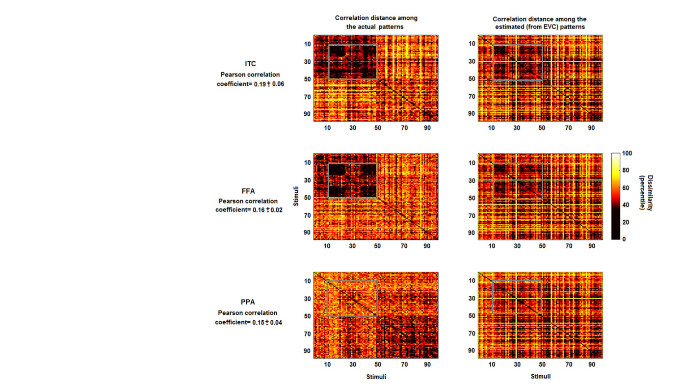
图 6 · 稀疏度估计:三对映射都超过 80%
原文图注:Fig 6. Estimated sparsity for the pattern transformation. The three panels show the estimates of the percentage of sparsity for the pattern transformations EVC->ITC, EVC->FFA and EVC->PPA, respectively. The dotted lines represent the mean RDD and GOF values across the simulation-realisations for each of the simulated percentages of sparsity, i.e. 50%, 60%, 70%, 80%, 90% and 99%. Each area between two dotted lines thus represents a fixed range for the percentage of sparsity, e.g. the area between the two curves associated with the blues and red squares denotes a degree of sparsity between 80% and 90%. The black squares (and their error bars) in the panels denote the mean (and the standard error of the mean) estimate of RDD and GOF across the four subjects. All estimates show a high percentage of sparsity for all transformations (>80%). Slightly higher percentages are shown by the transformations EVC->FFA and EVC->PPA.
各面板横轴为 GOF,纵轴为 RDD,虚线簇代表蒙特卡洛模拟针对 6 档稀疏度(50%–99%)生成的参照曲线,黑色方块及误差线表示 4 名被试的均值与标准误。实测落点显示:EVC→ITC 位于 80% 与 90% 参照线之间,EVC→PPA 位于 90% 以上区间。各被试间的误差范围相对较宽,表明稀疏度在统计上显著高于基线,但无法支持严格一对一连接的假设。
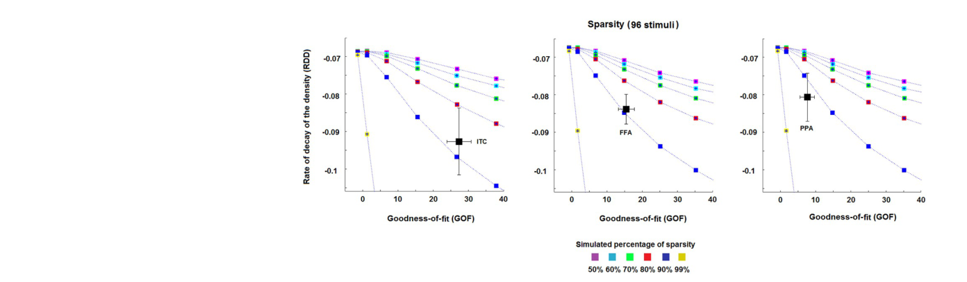
图 7 · 形变估计:FFA 最均匀,ITC 与 PPA 形变大
原文图注:Fig 7. Pattern deformation for each pair of ROIs. The three panels show the estimates of the rate of decay of SV-curve (RDSV), denoting the pattern deformation, of EVC->ITC, EVC->FFA and EVC->PPA for the 96 stimuli. The dotted lines represent the mean RDSV and GOF values across the simulation-realisations for each of the simulated rates of decay. Each area between two dotted lines thus represents a fixed range for the rate of decay. The black squares (and their error bars) in the panels denote the mean (and the standard error of the mean) estimate of RDSV and GOF across the four subjects.
图表格式与图 6 类似,参照曲线对应四档设定的奇异值衰减率(0、−0.01、−0.1、−1)。EVC→FFA 的实测均值落在 0 与 −0.01 曲线重合区间,提示其几何形变相对均匀;EVC→ITC 与 EVC→PPA 则落在 −0.1 及更陡峭区间,表现出各向异性的维度压缩与拉伸。作者指出,由于样本量限制,该指标在更精细生理差异上的验证仍依赖更大样本与更高信噪比的数据。
讨论
作者从三个层面讨论了研究的推断边界与方法特性。第一,关于线性模型的有效性:尽管皮层间的真实信号传递具有动态和非线性特征,当前实证表明线性估计足以解释显著方差并复现类别拓扑偏好;相比人工神经网络等黑盒非线性模型,线性变换允许直接提取稀疏度与几何形变等明确特征。第二,关于体素空间估计的必要性:选择在原生体素空间而非主成分空间估计变换,原因在于降维投影可能破坏局部拓扑对应,补充模拟(S7 图)表明体素空间的稀疏连接经 PCA 转换后稀疏性会显著丢失;作者同时测试了 LASSO 与弹性网络(elastic net),发现其平滑特异性容易在非稀疏真值下依然产生过度稀疏解(实测弹性网络所得矩阵稀疏度均超过 90%),因而推荐采用岭回归配合模拟校准。第三,关于研究局限与拓展:4 名被试的样本规模仅支持概念验证性质的推断;模型预设了前馈映射方向,未纳入反馈调节机制;后续可结合超对齐(hyperalignment)解决被试间体素空间解剖不对应问题,或引入因果建模推断方向性,亦可将框架扩展至静息态、MEG/EEG 时间序列以及多脑区偏回归分析。该研究的 MATLAB 分析代码已在 GitHub 开源。
一句话总结
该研究的核心方法学贡献在于将多体素功能连接从标量相关系数推进至映射矩阵层面,并建立了拟合优度、稀疏度和模式形变三个可定量的几何指标。4 名被试的小样本限制了生理结论的外推,但其实证流程为高维神经表征变换分析提供了结合模拟校准的操作框架。